From the transfer function to the frequency response
We have seen that for LTI systems whose output is a weighted sum of a finite number of past inputs and outputs, the transfer function amounts to being a rational function of the form
$H(z)=\frac{b_0 + b_1 z^{-1} + b_2 z^{-2} + \cdots b_M z^{-M}}{1+a_1 z^{-1} + a_2 z^{-2} + \cdots + a_Nz^{-N}}$or equivalently,
$\frac{z^{-M}b_0(z-\zeta_1)(z-\zeta_2)\cdots(z-\zeta_M)}{z^{-N}(z-p_1)(z-p_2)\cdots(z-p_N)}$One of the benefits in expressing the transfer function as the products of those single order polynomials is the elegant way it leads to understanding the magnitude of the transfer function:
$|H(z)|=\frac{|z^{-M}||b_0||(z-\zeta_1)||(z-\zeta_2)|\cdots|(z-\zeta_M)|}{|z^{-N}||(z-p_1)||(z-p_2)|\cdots|(z-p_N)|}$Note what terms like $|z-p|$ represent. The magnitude is $\sqrt{(Re(z)-Re(p))^2+(Im(z)-Im(p))^2}$ which is simply the euclidean distance between $z$ and $p$ on the complex plane. So the magnitude of the transfer function at some point $z$ essentially amounts to being the products of the distances between $z$ and the system's zeros, divided by the products of the distances between $z$ and the system's poles. The closer $z$ is to a zero, the smaller the magnitude of the transfer function will be; the closer $z$ is to a pole, the larger the magnitude of the transfer function will be.
Now recall that a system's frequency response, i.e. the amount the system scales the input at particular frequencies, is simply the z-transform evaluated on the unit circle, for $H(e^{j\omega})=H(z)|_{z=e^{j\omega}}$. If we have a pole-zero plot, we can quickly visualize the magnitude of the system's frequency response by traversing around the unit circle. As we go, the closer we are to a zero, the smaller it will be, while the closer we are to a pole, the larger it will be. As a result of this phenomenon (and the fact that the transfer function is determined by the pole and zero locations), we can see that the locations of a system's poles and zeros in the z-plane totally characterize a system (within a scaling factor). Thus, knowing the poles and zeros of a system is essentially equivalent to knowing exactly what kind of system it is.
Visualizing the magnitude of the frequency response
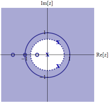
Consider the pole-zero plot from the example above, with a unit circle overlaid:
CAPTION. The frequency response of this system is simply value of the transfer function, evaluated along this unit circle. The magnitude of the transfer function is the product of the distances to the zeros, divided by the product of the distances to the poles. By traversing along the unit circle and noting these distances, we can visualize what the magnitude of the frequency response will be.
We will start at $\omega=0$. Here we can easily find the value of the magnitude, since $H(e^{j0})=H(1)$. From the transfer function we found in the first example, we have $H(1)=\frac{(1+3+\frac{11}{4}+\frac{3}{4})}{(1-1+\frac{1}{2})}=15$. So $|H(e^{j\omega})$ at $\omega=0$ is $15$. Now, as we move counter-clockwise around the circle (i.e., from $\omega=0$ to $\omega=\pi/2$ to $\omega=\pi$), note what happens. As $\omega$ approaches $\pi/4$ on the unit circle, it is drawing nearer and nearer to a pole; therefore, the magnitude of the frequency response is going to increase as $\omega$ progresses from $0$ to $\pi/4$. At that point, we will be travelling away from that pole, and nearer to the three zeros; accordingly, the magnitude of the frequency response will decrease. Eventually we will actually land squarely on a zero at $\omega=\pi$; this is obviously as close as we could possibly get to a zero. As the distance to the zero at that point is zero, the magnitude of the frequency response there is zero. We can repeat this process moving clockwise from $\omega=0$ to $\omega=-\pi$ and the magnitude will change in the precisely same way, due to the symmetry. Having moved along the entire unit circle, we can see how our intuition matches what is indeed the magnitude of the frequency response, found via plotting software:
CAPTION. Note that the magnitude is $15$ at $\omega=0$, then increases to a peak at about $\pm\pi/4$, and then decreases to $0$ as $\omega$ traverses from $\pm\pi/4$ to $\pm\pi$.
The transfer function roc, and stability
It has been explained previously that the region of convergence of a z-transform are the $z$ for which the sum $\sum x[n] z^{-n}$ converges. There is an alternative, though related definition that is also often used in signal processing, that the region of convergence are $z$ for which the sum $\sum x[n]z^{-n}$ converges ABSOLUTELY, i.e. that $\sum |x[n] z^{-n}|$. For virtually all of the signals that we will be considering, those two definitions are equivalent. The reason the second definition is often used is because of a relationship it establishes with the stability of the system.
Suppose that a system's transfer function $H(z)$ has a particular ROC (defined in the absolutely summable sense). If the unit circle ($|z|=1$) is contained by this ROC, then the system is BIBO stable. To prove this fact, we see simply that the $|z|=1$ being in the ROC means that $\sum |h[n]e^{j\omega}|$ converges for all $\omega$, and then note that for $\omega=0$, the convergent sum is $\sum |h[n]|$. Previously we proved that for LTI systems, $\sum |h[n]|$ converging is equivalent to the system being BIBO stable.
So if the unit circle is in a transfer function's ROC, then that system is BIBO stable. This is a helpful way to determine stability. We do not need to prove that an arbitrary bounded input will produce a bounded output, nor find the impulse response and determine its absolute summability; we simply need to know the transfer function's ROC.
If the system in question is causal (which is the case for most all practical systems of interest), then the ROC will extend outwards from the outermost pole. This means that, for causal systems, the location of the poles also determine BIBO stability. If all of a causal system's poles lie within the unit circle, then the ROC will extend to include the unit circle, and hence the system will be BIBO stable.
Stability and the pole/zero plot
Consider again the pole/zero plot from the system in the previous examples:
CAPTION. Since the ROC contains the $|z|=1$ unit circle, this system is BIBO stable.
Poles/zeros and fir/iir systems
We have seen that the poles and zeros of a system characterize it, which of course includes the nature of its frequency response and whether or not the system is BIBO stable. Given how significant the poles and zeros of a system are, it should come as no surprise that knowing about the poles and zeros also allows us to determine whether the system is FIR or IIR.
Put simply, if a system's transfer function has any poles (other than at $z=0$), then the system is IIR. If it has only zeros, then it is FIR. This follows from what we saw with regard to the nature of different kinds of ROCs. If the ROC is the entire $z$ plane (with the possible exception of $z=0$), then the impulse response is of finite duration; hence the system is FIR. But if there are any non-zero poles on the plane, than the ROC will either be a disk, an annulus, or will extend outside of a disk; in each of those cases, the impulse response is of infinite duration.