One of the most general ways of defining an LTI system is by expressing its output at some time $n$ as a weighted sum of values of the input and output at a finite number various other times. If all those times are at or prior to $n$, such systems a system is causal. In terms of a difference equation, the system definition would look something like this:
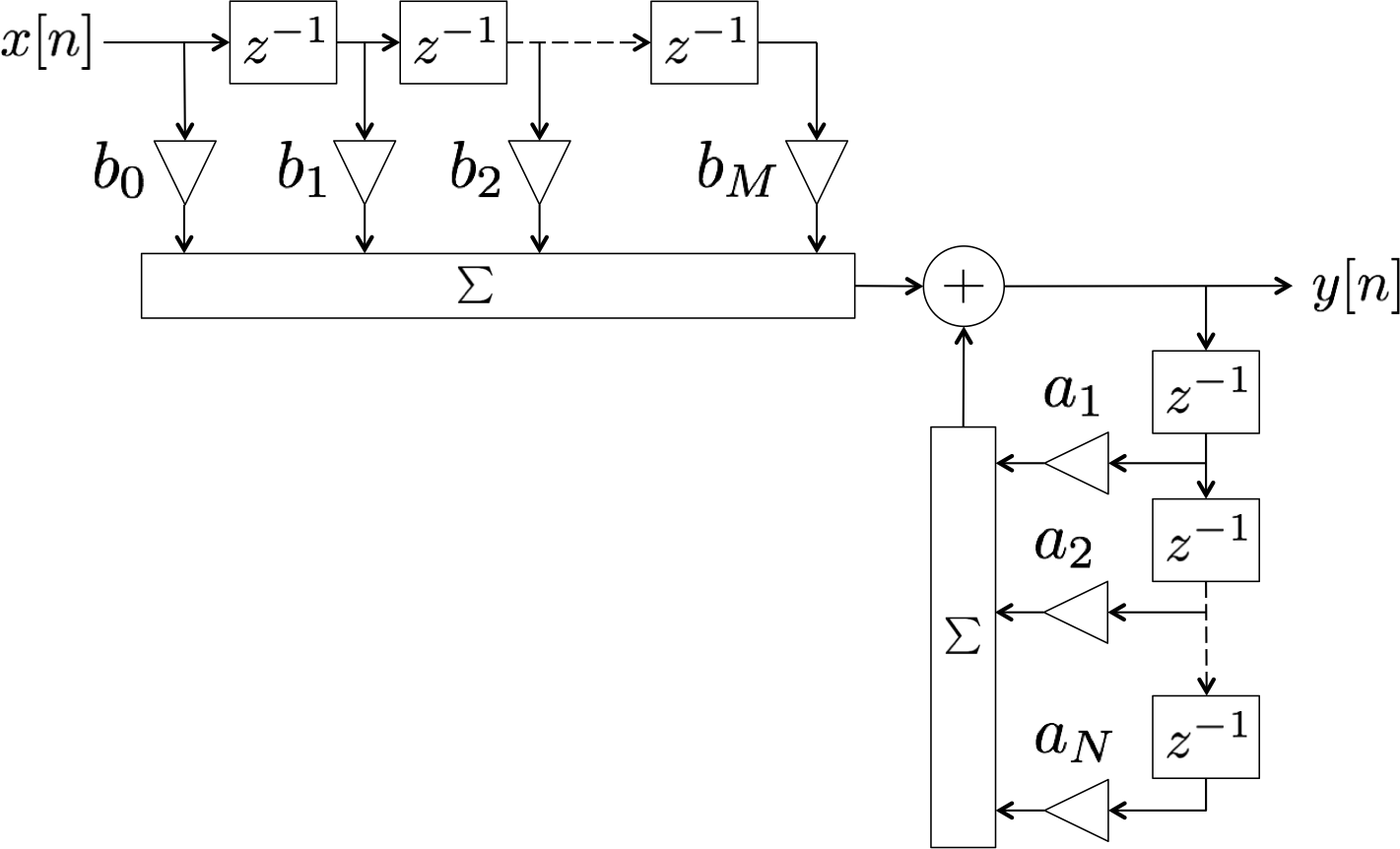
$y[n]~=~ b_0 x[n] + b_1 x[n-1]+ b_2 x[n-2] + \cdots + b_M x[n-M]-a_1 y[n-1] - a_2 y[n-2]+ \cdots - a_N y[n-N]$This kind of system can also be displayed as a block diagram:
CAPTION. In the block diagram, the $z^{-1}$ blocks represent time delays, the triangles represent multiplications, and the $\Sigma$ blocks represent summations of the signals being input into them. The output at time $n$ is a weighted sum of the previous $M$ input values (along with the current value) and previous $N$ output values.
Lti systems in the z-domain
Consider again the input/output relationship of a causal LTI system:
$y[n]~=~ b_0 x[n] + b_1 x[n-1]+ b_2 x[n-2] + \cdots + b_M x[n-M]-a_1 y[n-1] - a_2 y[n-2]+ \cdots - a_N y[n-N]$We can take the z-transform of this whole equation, bearing in mind that the transform is a linear operation and that delays of $n_0$ in time correspond to multiplications by $z^{-n_0}$ in the z-domain. That would leave us with this:
$Y(z)=~ b_0 X(z) + b_1 z^{-1} X(z) + b_2 z^{-2} X(z) + \cdots b_M z^{-M} X(z)- a_1 z^{-1} Y(z) - a_2 z^{-2} Y(z) - \cdots - a_N z^{-N} Y(z)$From there we can do a little rearranging:
$\begin{align*}Y(z)&=b_0 X(z) + b_1 z^{-1} X(z) + b_2 z^{-2} X(z) + \cdots b_M z^{-M} X(z)- a_1 z^{-1} Y(z) - a_2 z^{-2} Y(z) - \cdots - a_N z^{-N} Y(z)\\
Y(z)+ a_1 z^{-1} Y(z) a_2 z^{-2} Y(z) + \cdots + a_N z^{-N} Y(z)&=b_0 X(z) + b_1 z^{-1} X(z) + b_2 z^{-2} X(z) + \cdots b_M z^{-M}X(z)\\
Y(z)(1+a_1 z^{-1} + a_2 z^{-2} + \cdots + a_Nz^{-N})&=X(z)(b_0 + b_1 z^{-1} + b_2 z^{-2} + \cdots b_M z^{-M})\\
H(z)=\frac{Y(z)}{X(z)}&=\frac{b_0 + b_1 z^{-1} + b_2 z^{-2} + \cdots b_M z^{-M}}{1+a_1 z^{-1} + a_2 z^{-2} + \cdots + a_Nz^{-N}}
\end{align*}$This $H(z)$, which is a rational function in terms of $z$, is called the system's
transfer function .
The transfer function: poles and zeroes, roc, and stability
So we see that the transfer function for one of the most common classes of LTI systems--in which the output is a weighted sum of a finite number of past inputs and outputs--is a rational function in terms of $z$:
$H(z)=\frac{b_0 + b_1 z^{-1} + b_2 z^{-2} + \cdots b_M z^{-M}}{1+a_1 z^{-1} + a_2 z^{-2} + \cdots + a_Nz^{-N}}$We can express this function in terms of positive powers of $z$ by simple factoring, and then according to the fundamental theorem of algebra, we can represent the numerator and denominator polynomials with respect to their roots:
$\begin{align*}H(z)&=\frac{b_0 + b_1 z^{-1} + b_2 z^{-2} + \cdots b_M z^{-M}}{1+a_1 z^{-1} + a_2 z^{-2} + \cdots + a_Nz^{-N}}\\&=\frac{z^{-M}(b_0z^M+b_1z^{M-1}+b_2z^{M-2}+\cdots+b_M)}{z^{-N}(z^N+a_1z^{N-1}+a_2z^{N-2}+\cdots+a_N)}\\&=\frac{z^{-M}b_0(z-\zeta_1)(z-\zeta_2)\cdots(z-\zeta_M)}{z^{-N}(z-p_1)(z-p_2)\cdots(z-p_N)}
\end{align*}$The values of $z$ for which the numerator is zero are called
zeros , and the values for which the denominator is zero are called
poles .