<< Chapter < Page Chapter >> Page >

Additional general information can be obtained from [link] and the expression for a straight line, y = mx + b size 12{y= ital "mx"+b} {} .

In this case, the vertical axis y size 12{y} {} is V size 12{V} {} , the intercept b size 12{b} {} is v 0 size 12{v rSub { size 8{0} } } {} , the slope m size 12{m} {} is a size 12{a} {} , and the horizontal axis x size 12{x} {} is t size 12{t} {} . Substituting these symbols yields

v = v 0 + at . size 12{v=v rSub { size 8{0} } + ital "at"} {}

A general relationship for velocity, acceleration, and time has again been obtained from a graph. Notice that this equation was also derived algebraically from other motion equations in Motion Equations for Constant Acceleration in One Dimension .

It is not accidental that the same equations are obtained by graphical analysis as by algebraic techniques. In fact, an important way to discover physical relationships is to measure various physical quantities and then make graphs of one quantity against another to see if they are correlated in any way. Correlations imply physical relationships and might be shown by smooth graphs such as those above. From such graphs, mathematical relationships can sometimes be postulated. Further experiments are then performed to determine the validity of the hypothesized relationships.

Graphs of motion where acceleration is not constant

Now consider the motion of the jet car as it goes from 165 m/s to its top velocity of 250 m/s, graphed in [link] . Time again starts at zero, and the initial displacement and velocity are 2900 m and 165 m/s, respectively. (These were the final displacement and velocity of the car in the motion graphed in [link] .) Acceleration gradually decreases from 5 . 0 m/s 2 to zero when the car hits 250 m/s. The slope of the x vs. t graph increases until t = 55 s size 12{t="55"`s} {} , after which time the slope is constant. Similarly, velocity increases until 55 s and then becomes constant, since acceleration decreases to zero at 55 s and remains zero afterward.

Three line graphs of jet car displacement, velocity, and acceleration, respectively. First line graph is of position over time. Line is straight with a positive slope. Second line graph is of velocity over time. Line graph has a positive slope that decreases over time and flattens out at the end. Third line graph is of acceleration over time. Line has a negative slope that increases over time until it flattens out at the end. The line is not smooth, but has several kinks.
Graphs of motion of a jet-powered car as it reaches its top velocity. This motion begins where the motion in [link] ends. (a) The slope of this graph is velocity; it is plotted in the next graph. (b) The velocity gradually approaches its top value. The slope of this graph is acceleration; it is plotted in the final graph. (c) Acceleration gradually declines to zero when velocity becomes constant.

Calculating acceleration from a graph of velocity versus time

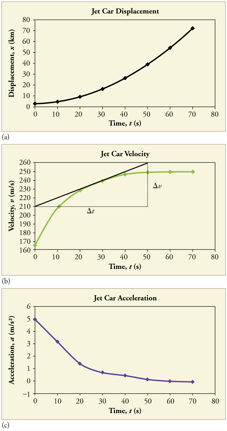
Calculate the acceleration of the jet car at a time of 25 s by finding the slope of the v size 12{v} {} vs. t size 12{t} {} graph in [link] (b).

Strategy

The slope of the curve at t = 25 s size 12{t="25"`s} {} is equal to the slope of the line tangent at that point, as illustrated in [link] (b).

Solution

Determine endpoints of the tangent line from the figure, and then plug them into the equation to solve for slope, a size 12{a} {} .

slope = Δ v Δ t = 260 m/s 210 m/s 51 s 1.0 s
a = 50 m/s 50 s = 1 . 0 m /s 2 .

Discussion

Note that this value for a is consistent with the value plotted in [link] (c) at t = 25 s size 12{t="25"`s} {} .

Got questions? Get instant answers now!

A graph of displacement versus time can be used to generate a graph of velocity versus time, and a graph of velocity versus time can be used to generate a graph of acceleration versus time. We do this by finding the slope of the graphs at every point. If the graph is linear (i.e., a line with a constant slope), it is easy to find the slope at any point and you have the slope for every point. Graphical analysis of motion can be used to describe both specific and general characteristics of kinematics. Graphs can also be used for other topics in physics. An important aspect of exploring physical relationships is to graph them and look for underlying relationships.

Questions & Answers

Ayele, K., 2003. Introductory Economics, 3rd ed., Addis Ababa.
Widad Reply
can you send the book attached ?
Ariel
?
Ariel
What is economics
Widad Reply
the study of how humans make choices under conditions of scarcity
AI-Robot
U(x,y) = (x×y)1/2 find mu of x for y
Desalegn Reply
U(x,y) = (x×y)1/2 find mu of x for y
Desalegn
what is ecnomics
Jan Reply
this is the study of how the society manages it's scarce resources
Belonwu
what is macroeconomic
John Reply
macroeconomic is the branch of economics which studies actions, scale, activities and behaviour of the aggregate economy as a whole.
husaini
etc
husaini
difference between firm and industry
husaini Reply
what's the difference between a firm and an industry
Abdul
firm is the unit which transform inputs to output where as industry contain combination of firms with similar production 😅😅
Abdulraufu
Suppose the demand function that a firm faces shifted from Qd  120 3P to Qd  90  3P and the supply function has shifted from QS  20  2P to QS 10  2P . a) Find the effect of this change on price and quantity. b) Which of the changes in demand and supply is higher?
Toofiq Reply
explain standard reason why economic is a science
innocent Reply
factors influencing supply
Petrus Reply
what is economic.
Milan Reply
scares means__________________ends resources. unlimited
Jan
economics is a science that studies human behaviour as a relationship b/w ends and scares means which have alternative uses
Jan
calculate the profit maximizing for demand and supply
Zarshad Reply
Why qualify 28 supplies
Milan
what are explicit costs
Nomsa Reply
out-of-pocket costs for a firm, for example, payments for wages and salaries, rent, or materials
AI-Robot
concepts of supply in microeconomics
David Reply
economic overview notes
Amahle Reply
identify a demand and a supply curve
Salome Reply
i don't know
Parul
there's a difference
Aryan
Demand curve shows that how supply and others conditions affect on demand of a particular thing and what percent demand increase whith increase of supply of goods
Israr
Hi Sir please how do u calculate Cross elastic demand and income elastic demand?
Abari
Got questions? Join the online conversation and get instant answers!
Jobilize.com Reply
Practice Key Terms 4

Get Jobilize Job Search Mobile App in your pocket Now!

Get it on Google Play Download on the App Store Now


Source:  OpenStax, College physics. OpenStax CNX. Jul 27, 2015 Download for free at http://legacy.cnx.org/content/col11406/1.9
Google Play and the Google Play logo are trademarks of Google Inc.

Notification Switch

Would you like to follow the 'College physics' conversation and receive update notifications?

Ask