5.2 Double integrals over general regions (Page 3/12)

Calculus volume 3 Page 3 / 12

Evaluating an iterated integral over a type i region

Evaluate the integral $\iint_{D} x^{2} e^{x y} d A$ where $D$ is shown in [link] .

First construct the region $D$ as a Type I region ( [link] ). Here $D = {(x, y) | 0 \leq x \leq 2, \frac{1}{2} x \leq y \leq 1} .$ Then we have

\iint_{D} x^{2} e^{x y} d A = \int_{x = 0}^{x = 2} \int_{y = 1 / 2 x}^{y = 1} x^{2} e^{x y} d y d x .

A triangle marked D drawn with lines y = 1/2 x and y = 1, with vertices (0, 0), (2, 1), and (0, 1). Here, there is a pair of red arrows reaching vertically from one edge to the other. — We can express region $D$ as a Type I region and integrate from $y = \frac{1}{2} x$ to $y = 1,$ between the lines $x = 0 and x = 2 .$

Therefore, we have

\begin{matrix} \int_{x = 0}^{x = 2} \int_{y = \frac{1}{2} x}^{y = 1} x^{2} e^{x y} d y d x & = \int_{x = 0}^{x = 2} [\int_{y = 1 / 2 x}^{y = 1} x^{2} e^{x y} d y] d x & Iterated integral for a Type I region. \\ = \int_{x = 0}^{x = 2} {[x^{2} \frac{e^{x y}}{x}] |}_{y = 1 / 2 x}^{y = 1} d x & \begin{matrix} Integrate with respect to y using \\ u -substitution with u = x y where x is held \\ constant. \end{matrix} \\ = \int_{x = 0}^{x = 2} [x e^{x} - x e^{x^{2} / 2}] d x & \begin{matrix} Integrate with respect to x using \\ u -substitution with u = \frac{1}{2} x^{2} . \end{matrix} \\ = {[x e^{x} - e^{x} - e^{\frac{1}{2} x^{2}}] |}_{x = 0}^{x = 2} = 2 \end{matrix}

Got questions? Get instant answers now!

In [link] , we could have looked at the region in another way, such as $D = {(x, y) | 0 \leq y \leq 1, 0 \leq x \leq 2 y}$ ( [link] ).

A triangle marked D drawn with lines x = 2y and y = 1, with vertices (0, 0), (2, 1), and (0, 1). Here there is a pair of red arrows reaching horizontally from one edge to the other.

This is a Type II region and the integral would then look like

\iint_{D} x^{2} e^{x y} d A = \int_{y = 0}^{y = 1} \int_{x = 0}^{x = 2 y} x^{2} e^{x y} d x d y .

However, if we integrate first with respect to $x,$ this integral is lengthy to compute because we have to use integration by parts twice.

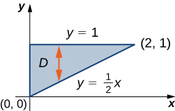
Evaluating an iterated integral over a type ii region

Evaluate the integral $\iint_{D} (3 x^{2} + y^{2}) d A$ where $= {(x, y) | - 2 \leq y \leq 3, y^{2} - 3 \leq x \leq y + 3} .$

Notice that $D$ can be seen as either a Type I or a Type II region, as shown in [link] . However, in this case describing $D$ as Type $I$ is more complicated than describing it as Type II. Therefore, we use $D$ as a Type II region for the integration.

This figure consists of two figures labeled a and b. In figure a, a region is bounded by y = the square root of the quantity (x + 3), y = the negative of the square root of the quantity (x + 3), and y = x minus 3, which has points of intersection (6, 3), (1, negative 2), and (0, negative 3). There are vertical lines in the shape, and it is noted that this is a type I region: integrate first with respect to y. In figure b, a region is bounded by x = y2 minus 3 and x = y + 3, which has points of intersection (6, 3), (1, negative 2), and (0, negative 3). There are horizontal lines in the shape, and it is noted that this is a type II region: integrate first with respect to x. — The region $D$ in this example can be either (a) Type I or (b) Type II.

Choosing this order of integration, we have

\begin{matrix} \iint_{D} (3 x^{2} + y^{2}) d A & = \int_{y = −2}^{y = 3} \int_{x = y^{2} - 3}^{x = y + 3} (3 x^{2} + y^{2}) d x d y & Iterated integral, Type II region. \\ = {\int_{y = −2}^{y = 3} (x^{3} + x y^{2}) |}_{y^{2} - 3}^{y + 3} d y & Integrate with respect to x . \\ = \int_{y = −2}^{y = 3} ({(y + 3)}^{3} + (y + 3) y^{2} - {(y^{2} - 3)}^{3} - (y^{2} - 3) y^{2}) d y \\ = \int_{−2}^{3} (54 + 27 y - 12 y^{2} + 2 y^{3} + 8 y^{4} - y^{6}) d y & Integrate with respect to y . \\ = {[54 y + \frac{27 y^{2}}{2} - 4 y^{3} + \frac{y^{4}}{2} + \frac{8 y^{5}}{5} - \frac{y^{7}}{7}] |}_{−2}^{3} \\ = \frac{2375}{7} . \end{matrix}

Got questions? Get instant answers now!

Sketch the region $D$ and evaluate the iterated integral $\iint_{D} x y d y d x$ where $D$ is the region bounded by the curves $y = cos x$ and $y = sin x$ in the interval $[−3 π / 4, π / 4] .$

$π / 4$

Got questions? Get instant answers now!

Recall from Double Integrals over Rectangular Regions the properties of double integrals. As we have seen from the examples here, all these properties are also valid for a function defined on a nonrectangular bounded region on a plane. In particular, property $3$ states:

If $R = S \cup T$ and $S \cap T = \emptyset$ except at their boundaries, then

\iint_{R} f (x, y) d A = \iint_{S} f (x, y) d A + \iint_{T} f (x, y) d A .

Similarly, we have the following property of double integrals over a nonrectangular bounded region on a plane.

Decomposing regions into smaller regions

Suppose the region $D$ can be expressed as $D = D_{1} \cup D_{2}$ where $D_{1}$ and $D_{2}$ do not overlap except at their boundaries. Then

\iint_{D} f (x, y) d A = \iint_{D_{1}} f (x, y) d A + \iint_{D_{2}} f (x, y) d A .

This theorem is particularly useful for nonrectangular regions because it allows us to split a region into a union of regions of Type I and Type II. Then we can compute the double integral on each piece in a convenient way, as in the next example.

Decomposing regions

Express the region $D$ shown in [link] as a union of regions of Type I or Type II, and evaluate the integral

\iint_{D} (2 x + 5 y) d A .

A complicated shape enclosed by the lines y = (x + 2) squared, x = 16y minus y cubed, x = negative 2, and y = negative 4. This graph has intersection points (0, 4), (negative 2, 0), (0, negative 4), and (negative 2, negative 4). — This region can be decomposed into a union of three regions of Type I or Type II.

The region $D$ is not easy to decompose into any one type; it is actually a combination of different types. So we can write it as a union of three regions $D_{1}, D_{2}, and D_{3}$ where, $D_{1} = {(x, y) | - 2 \leq x \leq 0, 0 \leq y \leq {(x + 2)}^{2}},$ $D_{2} = {(x, y) | 0 \leq y \leq 4, 0 \leq x \leq (y - \frac{1}{16} y^{3})} .$ These regions are illustrated more clearly in [link] .

The same complicated shape enclosed by the lines y = (x + 2) squared, x = 16y minus y cubed, x = negative 2, and y = negative 4. This graph has intersection points (0, 4), (negative 2, 0), (0, negative 4), and (negative 2, negative 4). The area in the first quadrant is marked as D2 and a Type II region. The region in the second quadrant is marked as D1 and is a Type I region. The region in the third quadrant is marked as D3 and is a Type II region. — Breaking the region into three subregions makes it easier to set up the integration.

Here $D_{1}$ is Type $I$ and $D_{2}$ and $D_{3}$ are both of Type II. Hence,

\begin{matrix} \iint_{D} (2 x + 5 y) d A & = \iint_{D_{1}} (2 x + 5 y) d A + \iint_{D_{2}} (2 x + 5 y) d A + \iint_{D_{3}} (2 x + 5 y) d A \\ = \int_{x = −2}^{x = 0} \int_{y = 0}^{y = {(x + 2)}^{2}} (2 x + 5 y) d y d x + \int_{y = 0}^{y = 4} \int_{x = 0}^{x = y - (1 / 16) y^{3}} (2 + 5 y) d x d y + \int_{y = −4}^{y = 0} \int_{x = −2}^{x = y - (1 / 16) y^{3}} (2 x + 5 y) d x d y \\ = \int_{x = −2}^{x = 0} [\frac{1}{2} {(2 + x)}^{2} (20 + 24 x + 5 x^{2})] + \int_{y = 0}^{y = 4} [\frac{1}{256} y^{6} - \frac{7}{16} y^{4} + 6 y^{2}] \\ + \int_{y = −4}^{y = 0} [\frac{1}{256} y^{6} - \frac{7}{16} y^{4} + 6 y^{2} + 10 y - 4] \\ = \frac{40}{3} + \frac{1664}{35} - \frac{1696}{35} = \frac{1304}{105} . \end{matrix}

Now we could redo this example using a union of two Type II regions (see the Checkpoint).

Got questions? Get instant answers now!

<< Chapter < Page Page > Chapter >>

Practice Key Terms 3

Read also:

Get Jobilize Job Search Mobile App in your pocket Now!

100% Free Mobile Applications
Receive real-time job alerts and never miss the right job again

Source: OpenStax, Calculus volume 3. OpenStax CNX. Feb 05, 2016 Download for free at http://legacy.cnx.org/content/col11966/1.2

Google Play and the Google Play logo are trademarks of Google Inc.

Notification Switch

Would you like to follow the 'Calculus volume 3' conversation and receive update notifications?

Ask

	2 Timeshare 2 By Jams Kalo Start Quiz
	24 Biology 24 Fungi MCQ By OpenStax Start Quiz
	Cultural Anthropology Definition By Richley Crapo Start Assignment
	2 Gastrointestinal Pathophysiology Self-Assessment By Laurence Bailen Start Assessment
	27 AP 27 Reproductive System MCQ By OpenStax Start Quiz
	How well do you know 5SOS? By Wey Hey Start Quiz
	3 Biology 03 Biological Macromolecules MCQ By OpenStax Start Quiz
	2 AP 02 Chemical Level of Organization Essay By OpenStax Start Flashcards
	3 Understanding Societies MCQ By Jessica Collett Start Quiz
	U.s. history By OpenStax Read Online Course