5.1 Double integrals over rectangular regions (Page 4/12)

Calculus volume 3 Page 4 / 12

Fubini’s theorem

Suppose that $f (x, y)$ is a function of two variables that is continuous over a rectangular region $R = {(x, y) \in ℝ^{2} | a \leq x \leq b, c \leq y \leq d} .$ Then we see from [link] that the double integral of $f$ over the region equals an iterated integral,

\iint_{R} f (x, y) d A = \iint_{R} f (x, y) d x d y = \int_{a}^{b} \int_{c}^{d} f (x, y) d y d x = \int_{c}^{d} \int_{a}^{b} f (x, y) d x d y .

More generally, Fubini’s theorem is true if $f$ is bounded on $R$ and $f$ is discontinuous only on a finite number of continuous curves. In other words, $f$ has to be integrable over $R .$

This figure consists of two figures marked a and b. In figure a, in xyz space, a surface is shown that is given by the function f(x, y). A point x is chosen on the x axis, and at this point, it it written fix x. From this point, a plane is projected perpendicular to the xy plane along the line with value x. This plane is marked Area A(x), and the entire space under the surface is marked V. Similarly, in figure b, in xyz space, a surface is shown that is given by the function f(x, y). A point y is chosen on the y axis, and at this point, it it written fix y. From this point, a plane is projected perpendicular to the xy plane along the line with value y. This plane is marked Area A(y), and the entire space under the surface is marked V. 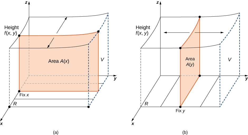— (a) Integrating first with respect to $y$ and then with respect to $x$ to find the area $A (x)$ and then the volume V ; (b) integrating first with respect to $x$ and then with respect to $y$ to find the area $A (y)$ and then the volume V .

Using fubini’s theorem

Use Fubini’s theorem to compute the double integral $\iint_{R} f (x, y) d A$ where $f (x, y) = x$ and $R = [0, 2] \times [0, 1] .$

Fubini’s theorem offers an easier way to evaluate the double integral by the use of an iterated integral. Note how the boundary values of the region R become the upper and lower limits of integration.

\begin{matrix} \iint_{R} f (x, y) d A & = \iint_{R} f (x, y) d x d y \\ = \int_{y = 0}^{y = 1} \int_{x = 0}^{x = 2} x d x d y \\ = \int_{y = 0}^{y = 1} [{\frac{x^{2}}{2} |}_{x = 0}^{x = 2}] d y \\ = \int_{y = 0}^{y = 1} 2 d y = {2 y |}_{y = 0}^{y = 1} = 2 . \end{matrix}

Got questions? Get instant answers now!

The double integration in this example is simple enough to use Fubini’s theorem directly, allowing us to convert a double integral into an iterated integral. Consequently, we are now ready to convert all double integrals to iterated integrals and demonstrate how the properties listed earlier can help us evaluate double integrals when the function $f (x, y)$ is more complex. Note that the order of integration can be changed (see [link] ).

Illustrating properties i and ii

Evaluate the double integral $\iint_{R} (x y - 3 x y^{2}) d A$ where $R = {(x, y) | 0 \leq x \leq 2, 1 \leq y \leq 2} .$

This function has two pieces: one piece is $x y$ and the other is $3 x y^{2} .$ Also, the second piece has a constant $3 .$ Notice how we use properties i and ii to help evaluate the double integral.

\begin{matrix} \iint_{R} (x y - 3 x y^{2}) d A \\ = \iint_{R} x y d A + \iint_{R} (−3 x y^{2}) d A & Property i: Integral of a sum is the sum of the integrals. \\ = \int_{y = 1}^{y = 2} \int_{x = 0}^{x = 2} x y d x d y - \int_{y = 1}^{y = 2} \int_{x = 0}^{x = 2} 3 x y^{2} d x d y & Convert double integrals to iterated integrals. \\ = \int_{y = 1}^{y = 2} {(\frac{x^{2}}{2} y) |}_{x = 0}^{x = 2} d y - 3 \int_{y = 1}^{y = 2} {(\frac{x^{2}}{2} y^{2}) |}_{x = 0}^{x = 2} d y & Integrate with respect to x, holding y constant. \\ = \int_{y = 1}^{y = 2} 2 y d y - \int_{y = 1}^{y = 2} 6 y^{2} d y & Property ii: Placing the constant before the integral. \\ = \int_{1}^{2} y d y - 6 \int_{1}^{2} y^{2} d y & Integrate with respect to y . \\ = {2 \frac{y^{2}}{2} |}_{1}^{2} - {6 \frac{y^{3}}{3} |}_{1}^{2} \\ = {y^{2} |}_{1}^{2} - {2 y^{3} |}_{1}^{2} \\ = (4 - 1) - 2 (8 - 1) \\ = 3 - 2 (7) = 3 - 14 = −11. \end{matrix}

Got questions? Get instant answers now!

Illustrating property v.

Over the region $R = {(x, y) | 1 \leq x \leq 3, 1 \leq y \leq 2},$ we have $2 \leq x^{2} + y^{2} \leq 13 .$ Find a lower and an upper bound for the integral $\iint_{R} (x^{2} + y^{2}) d A .$

For a lower bound, integrate the constant function 2 over the region $R .$ For an upper bound, integrate the constant function 13 over the region $R .$

\begin{matrix} \int_{1}^{2} \int_{1}^{3} 2 d x d y & = & \int_{1}^{2} [{2 x |}_{1}^{3}] d y = \int_{1}^{2} 2 (2) d y = {4 y |}_{1}^{2} = 4 (2 - 1) = 4 \\ \int_{1}^{2} \int_{1}^{3} 13 d x d y & = & \int_{1}^{2} [{13 x |}_{1}^{3}] d y = \int_{1}^{2} 13 (2) d y = {26 y |}_{1}^{2} = 26 (2 - 1) = 26. \end{matrix}

Hence, we obtain $4 \leq \iint_{R} (x^{2} + y^{2}) d A \leq 26 .$

Got questions? Get instant answers now!

Illustrating property vi

Evaluate the integral $\iint_{R} e^{y} cos x d A$ over the region $R = {(x, y) | 0 \leq x \leq \frac{π}{2}, 0 \leq y \leq 1} .$

This is a great example for property vi because the function $f (x, y)$ is clearly the product of two single-variable functions $e^{y}$ and $cos x .$ Thus we can split the integral into two parts and then integrate each one as a single-variable integration problem.

\begin{matrix} \iint_{R} e^{y} cos x d A & = \int_{0}^{1} \int_{0}^{π / 2} e^{y} cos x d x d y \\ = (\int_{0}^{1} e^{y} d y) (\int_{0}^{π / 2} cos x d x) \\ = ({e^{y} |}_{0}^{1}) ({sin x |}_{0}^{π / 2}) \\ = e - 1. \end{matrix}

Got questions? Get instant answers now!

<< Chapter < Page Page > Chapter >>

Practice Key Terms 4

Read also:

Get Jobilize Job Search Mobile App in your pocket Now!

100% Free Mobile Applications
Receive real-time job alerts and never miss the right job again

Source: OpenStax, Calculus volume 3. OpenStax CNX. Feb 05, 2016 Download for free at http://legacy.cnx.org/content/col11966/1.2

Google Play and the Google Play logo are trademarks of Google Inc.

Notification Switch

Would you like to follow the 'Calculus volume 3' conversation and receive update notifications?

Ask

	2 Human A&P 2- Test 2 By Madison Christian Start Flashcards
	21 Biology 21 Viruses MCQ By OpenStax Start Quiz
	1 Pharmacology Nervous System MCQ By Rohini Ajay Start Quiz
	Professional makeup certification Test By Angela January Start Quiz
	8 Biology 08 Photosynthesis MCQ By OpenStax Start Quiz
©flickr: Mike	Examples of Wiffle IQ By Sean WiffleBoy Start Quiz
	4 AP 04 Tissue Level of Organization Essay By OpenStax Start Flashcards
	2 Biology 02 The Chemical Foundation of Life MCQ By OpenStax Start Quiz
	6 Psychology MCQ 2010 2 Exam By John Gabrieli Start Exam
	5 BOD Reproductive System quiz By Brooke Delaney Start Quiz