

| << Chapter < Page | Chapter >> Page > |
| T(K) | K p |
| 500 | 6.25·10 -3 |
| 550 | 8.81·10 -3 |
| 650 | 1.49·10 -2 |
| 700 | 1.84·10 -2 |
| 720 | 1.98·10 -2 |
These data do not seem to give a simple relationship between K p and temperature. We must appeal to arguments based on Thermodynamics, which we will develop in a future Concept Development Study. From Thermodynamics, it is possible to show that the equilibrium constant should vary with temperature according to the following equation:
If ΔH˚ and ΔS˚ do not depend strongly on the temperature, then this equation would predict a simple straight line relationship between ln K p and 1/T . In addition, the slope of this line should be -ΔH˚/R . We test this possibility with the graph in Figure 4.
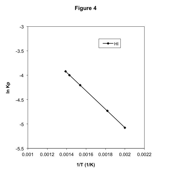
In fact, we do observe a straight line through the data. In this case, the line has a negative slope. Note carefully that this means that K p is increasing with temperature. The negative slope via Equation(14) means that -ΔH˚/R must be negative, and indeed for Reaction (3) in this temperature range, ΔH˚ = 15.6 kJ/mol. This value matches well with the slope of the line in Figure 4.
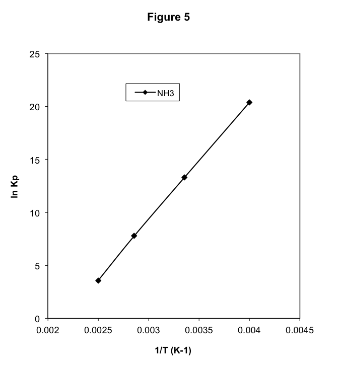
Given the validity of Equation (13) in describing the temperature dependence of the equilibrium constant, we should predict that an exothermic reaction with ΔH˚<0 should have a positive slope in the graph of ln K p versus 1/T . We thus predict that the equilibrium constant should decrease with increasing temperature. Let’s test this. A good example of an exothermic reaction is Reaction (2)
N 2 (g) + 3 H 2 (g) → 2 NH 3 (g)(2)
for which ΔH˚ = -92.2 kJ/mol. Equilibrium constant data are given in Table 5. Note that, as predicted, the equilibrium constant for this exothermic reaction decreases rapidly with increasing temperature. The data from Table 5 is shown in Figure 5, clearly showing the contrast between the endothermic reaction and the exothermic reaction. The slope of the graph is positive for the exothermic reaction and negative for the endothermic reaction. From Equation (13), this is a general result for all reactions.
| T(K) | K p |
|---|---|
| 250 | 7·10 8 |
| 298 | 6·10 5 |
| 350 | 2·10 3 |
| 400 | 36 |
One of our goals at the outset was to determine whether it is possible to control the equilibrium that occurs during a gas reaction. We might want to force a reaction to produce as much of the products as possible. In the alternative, if there are unwanted by-products of a reaction, we might want conditions that minimize the product. We have observed that the amount of product varies with the quantities of initial materials and with changes in the temperature. Our goal is a systematic understanding of these variations.
A look back at Tables 1 and 2 shows that the equilibrium pressure of the product of the reaction increases with increasing the initial quantity of reaction. This seems quite intuitive. Less intuitive is the variation of the equilibrium pressure of the product of Reaction (2) with variation in the volume of the container, as shown in Table 3. Note that the pressure of NH 3 decreases by more than a factor of ten when the volume is increased by a factor of ten. This means that, at equilibrium, there are fewer moles of NH 3 produced when the reaction occurs in a larger volume.
Notification Switch
Would you like to follow the 'Concept development studies in chemistry 2013' conversation and receive update notifications?

|
|

|
|

|
|

|
|

|
|

|
|
|
|
|

|
|

|
|

|