15.5 Pitfalls for monetary policy  (Page 4/20)

Changes in velocity can cause problems for monetary policy. To understand why, rewrite the definition of velocity so that the money supply is on the left-hand side of the equation. That is:

Recall from The Macroeconomic Perspective that

Therefore,

This equation is sometimes called the basic quantity equation of money    but, as you can see, it is just the definition of velocity written in a different form. This equation must hold true, by definition.

If velocity is constant over time, then a certain percentage rise in the money supply on the left-hand side of the basic quantity equation of money will inevitably lead to the same percentage rise in nominal GDP —although this change could happen through an increase in inflation, or an increase in real GDP    , or some combination of the two. If velocity is changing over time but in a constant and predictable way, then changes in the money supply will continue to have a predictable effect on nominal GDP. If velocity changes unpredictably over time, however, then the effect of changes in the money supply on nominal GDP becomes unpredictable.

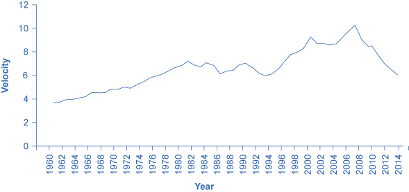
The actual velocity of money in the U.S. economy as measured by using M1, the most common definition of the money supply, is illustrated in [link] . From 1960 up to about 1980, velocity appears fairly predictable; that is, it is increasing at a fairly constant rate. In the early 1980s, however, velocity as calculated with M1 becomes more variable. The reasons for these sharp changes in velocity remain a puzzle. Economists suspect that the changes in velocity are related to innovations in banking and finance which have changed how money is used in making economic transactions: for example, the growth of electronic payments; a rise in personal borrowing and credit card usage; and accounts that make it easier for people to hold money in savings accounts, where it is counted as M2, right up to the moment that they want to write a check on the money and transfer it to M1. So far at least, it has proven difficult to draw clear links between these kinds of factors and the specific up-and-down fluctuations in M1. Given many changes in banking and the prevalence of electronic banking, M2 is now favored as a measure of money rather than the narrower M1.

Velocity calculated using m1

In the 1970s, when velocity as measured by M1 seemed predictable, a number of economists, led by Nobel laureate Milton Friedman (1912–2006), argued that the best monetary policy was for the central bank to increase the money supply at a constant growth rate. These economists argued that with the long and variable lags of monetary policy, and the political pressures on central bankers, central bank monetary policies were as likely to have undesirable as to have desirable effects. Thus, these economists believed that the monetary policy should seek steady growth in the money supply of 3% per year. They argued that a steady rate of monetary growth would be correct over longer time periods, since it would roughly match the growth of the real economy. In addition, they argued that giving the central bank less discretion to conduct monetary policy would prevent an overly activist central bank from becoming a source of economic instability and uncertainty. In this spirit, Friedman wrote in 1967: “The first and most important lesson that history teaches about what monetary policy can do—and it is a lesson of the most profound importance—is that monetary policy can prevent money itself from being a major source of economic disturbance.”