Having considered discrete-time signal types, systems and their properties, and various signal transformations that can assist with analysis, we are ready to put this knowledge to use. After all, signals and systems are not just interesting mathematical entities-- they are actually useful! Signals represent real-world information, and systems can perform a variety of important modifications on them.
Filtering: lti systems in the frequency domain
Before we can design a filter to meet some kind of desired specification, we first need to remind ourselves of what LTI systems can do. We will explain filtering from the standpoint of infinite-length signals, but the principles apply similarly to finite-length signals as well. Recall these two important facts: first, that any discrete-time signal can be represented as an integral of complex sinusoids, and second, that complex sinusoids are eigenvectors of LTI systems. Putting those facts together, we see that LTI can be understood as taking in discrete-time signals as inputs, and then modifying them by scaling their frequency components. The amount the system scales each frequency component $\omega$ is the system's frequency response $H(\omega)$. The frequency response is itself simply the DTFT of the system's impulse response $h[n]$.
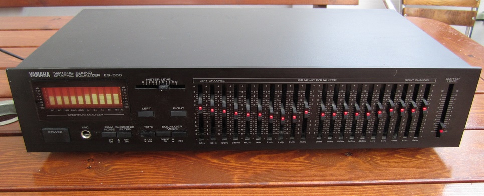
So, LTI systems work by taking in input signals and scaling each input frequency according to the system's frequency response in order to produce the output. In this way, they can be thought of as being (infinitesimally) finely scaled versions of a graphic equalizer, which modifies input music signals according to frequency bands.
The filtering operation of discrete-time LTI systems is similar to the frequency tuning of musical signals with a graphic equalizer. [https://www.flickr.com/photos/12577725@N05/6103827986] Yamaha EQ-500 by Touho_T, used under [http://creativecommons.org/licenses/by/2.0/]CC BY / cropped from original.
Since there is an infinite number of discrete-time frequencies $\omega$ (as it is a real number between $-\pi$ and $\pi$), and each one can be scaled in an infinite number of ways (since the scaling factor is any complex number), there are obviously an infinite number of potential filters/systems. That said, filters are usually categorized as being one of four different classes.
Filter types
The most common filter types are named according to the signal frequency components they either stop (scale by zero) or allow to pass. The magnitudes of their frequency response and their corresponding impulse responses are plotted below.
The frequency response magnitude and impulse response of a
low-pass filter . Note how the lowest frequencies (those near to $\omega=0$) are scaled by a (relatively) constant value, while the highest frequencies (those near $\omega=\pm\pi$) are attenuated.A
high-pass filter does the opposite of a low-pass filter; it attenuates lower frequencies and allows higher frequencies to pass.Plotted above are the frequency response magnitude and impulse response of a
band-pass filter . These filters allow a narrow (contiguous) band of frequencies to pass (here, those near $\omega=\pm\frac{\pi}{2}$) while attenuating the rest.A
band-stop filter , like the band-pass filter, also focuses on a narrow band of frequencies. But in this case, it attenuates that band, while allowing other frequencies to pass. As can be seen in the frequency responses above, the names of the typical filter classes give a straightforward description of the filters' function. Note, though, that there may be some level of ambiguity between filter names. For example, a low-pass filter is also a type of band-pass filter (with low frequencies being the "band"), and for that matter is also a band-stop filter (the high frequencies being the band that is stopped). We could say the same thing about high-pass filters, as well. In practice, then, band-pass and band-stop filters typically are understood to pass or stop bands that are not about $0$ or $\pi$, but some other frequency. Additionally, the pass and stop bands of these two filters are typically much narrower than those for high-pass or low-pass filters.
Filter design
Note the simplicity of the four filters plotted above; their impulse responses have only 2 or 4 non-zero values, and even those are either 1 or -1. In practice, discrete-time filters can have impulse response lengths that are much longer and more complex. The advantages of such filters is that their frequency pass- and stop- points are much sharper, with more level pass-bands. We can see this trade-off when comparing the frequency and impulse response of the low-pass filter above with the following "ideal" low-pass filter:
The frequency response magnitude and impulse response of an
ideal low-pass filter . We can see why this filter is called "ideal." For all of the frequencies below a certain point $\omega_c$, the filter scales them by 1, meaning it does not change their magnitude at all; then, for all frequencies higher than $\omega_c$, it perfectly zeroes them out. Of course, this comes at a cost: the impulse response of this filter ($h[n]=2 \omega_c \frac{\sin(\omega_c n)}{\omega_c n}$) is infinitely long and is not causal (meaning the system needs to know future values of the input to calculate the current value of the output). Furthermore, because its transfer function is not a rational function of finite order, it has infinite complexity, and thus cannot be perfectly implemented in practice.
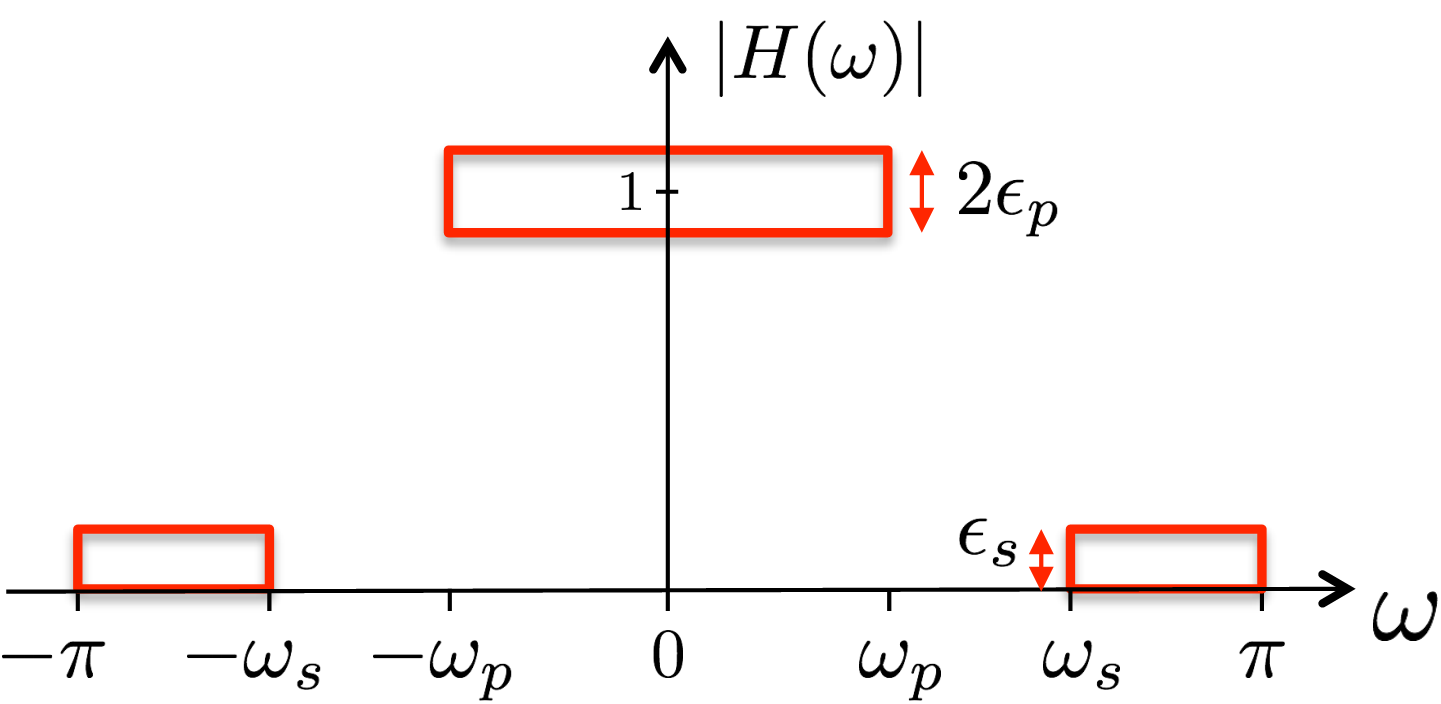
The task of filter design is to work with these two constraints, having a desirable frequency response without having an overly complex impulse response (which affects the complexity and cost of the filter's real-world implementation). The "desirability" of a filter's frequency response is typically expressed by giving certain constraints on its performance:
The performance constraints for filters are typically expressed as allowable deviations from $|H(\omega)|=1$ in the filter's pass-band (which is indicated by $\omega_p$) and from $|H(\omega)|=0$ in the stop-band (the "cutoff" of which is indicated by $\omega_c$). Within given filter design parameters, the simplest possible implementation is sought. There are two main approaches towards implementation, IIR and FIR; we will subsequently consider the characteristics, advantages, and disadvantages of each.