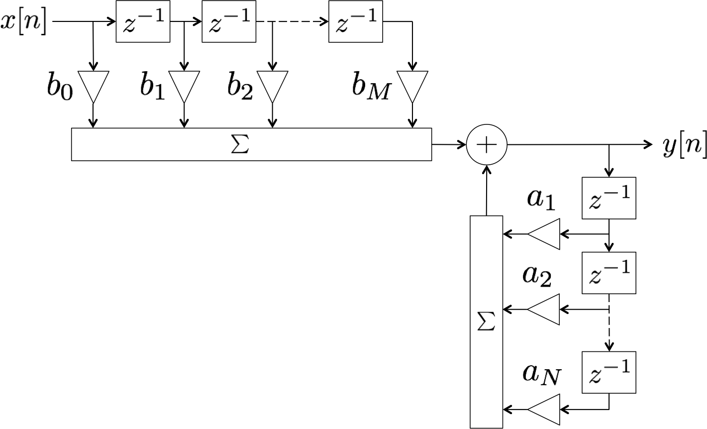
Recall the system representation of discrete-time LTI systems:
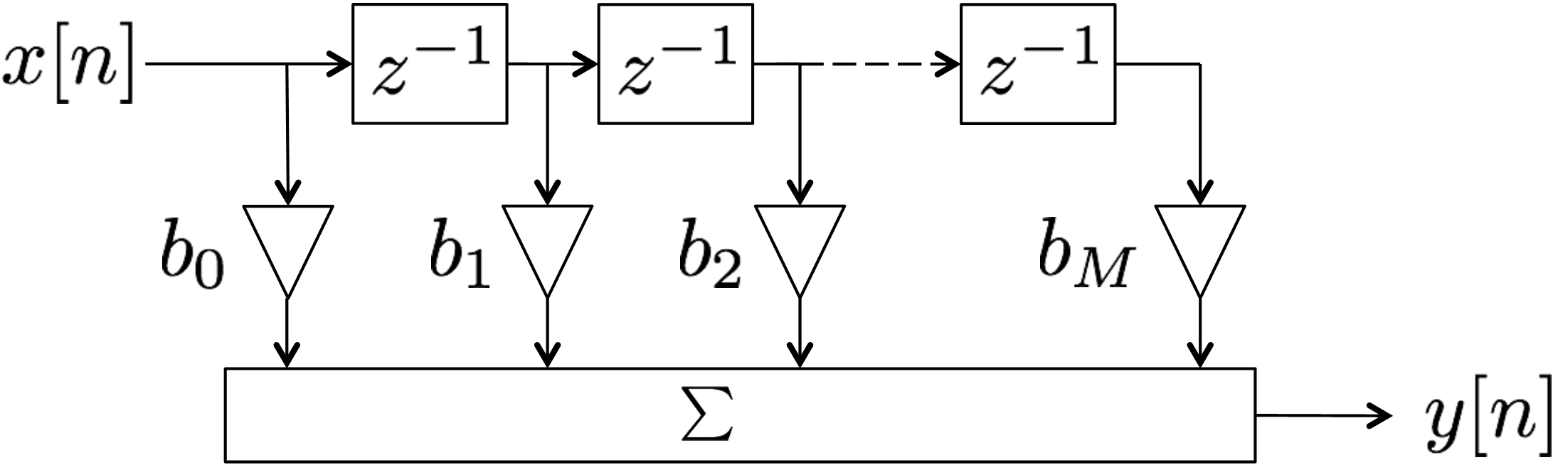
Implementation of a discrete-time LTI system. FIR systems are those that do not have poles/feedback, so the representation can be simplified:
Implementation of an FIR discrete-time LTI system. From the straightforward time domain expression of this kind of system ($y[n] = b_0 x[n]+ b_1 x[n-1]+ b_2 x[n-2]+ \cdots b_M x[n-M]$) we have the following transfer function:$\begin{align*} H(z)= \frac{Y(z)}{X(z)}&= b_0 + b_1 z^{-1} + b_2 z^{-2} + \cdots b_M z^{-M}\\&= z^{-M}(z-\zeta_1)(z-\zeta_2) \cdots (z-\zeta_M) \end{align*}$
In the z-domain, such systems have only zeros (not counting poles at $z=0$, or in the case of acausal systems, poles at $z=\infty$).
Fir filters
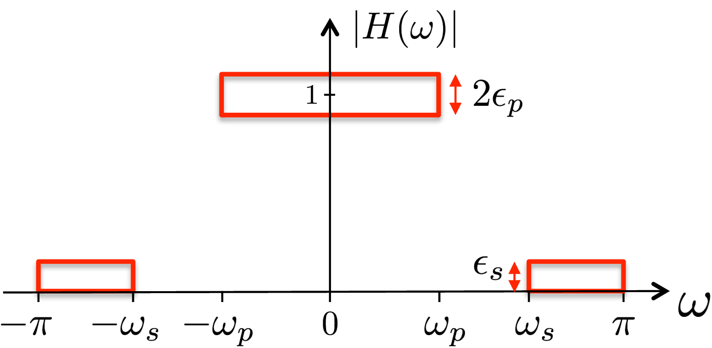
As FIR filters are FIR discrete-time LTI systems, their design is simply a matter of adjusting the $b$ coefficients of the time-domain representation (or equivalently, the location of the zeros in the z- domain). As with IIR systems, these systems are designed to perform to particular specifications in the frequency domain:
CAPTION. FIR filters must be of much higher order (i.e., have more non-zero coefficients in their time-domain representations) than IIR filters to achieve similar performance, but in exhange for this cost have several benefits over IIR filters. First, an FIR filter is GUARANTEED to be BIBO stable. Recalling that an LTI system is BIBO stable if and only if its impulse response is absolutely summable, the finite length of FIR impulse responses guarantees this condition. And second, unlike the non-linearity with IIR filters, FIR filters can be easily designed to have a
generalized linear phase response (a phase response that is linear, with one caveat; see below).
In order to have a generalized linear phase response, FIR filters of length $N$ must be designed so that their impulse responses $h[n]$ are either even or odd symmetric about the center time value(s) ($(N-1)/2$ for odd $n$, $n=N/2$ and $n=N/2-1$ for even $N$). This design can be attained for $N$ that are either even or odd. We will consider when $N$ is odd, i.e. when $N=M+1$ where $M$ is an even number. For such a filter length, evenness implies that $h[n]=h[M-n]$. Suppose the impulse response is designed so that such is the case. Let's take a look at the system's frequency response, using that symmetry to simplify things:$\begin{align*}
H(\omega)&= \sum_{n=0}^{M} h[n]e^{-j\omega n}\\&= \sum_{n=0}^{M/2-1} h[n]e^{-j\omega n} + h[M/2]e^{-j\omega M/2} +
\sum_{n=M/2+1}^{M} h[n]e^{-j\omega n}
\\&= \sum_{n=0}^{M/2-1} h[n]e^{-j\omega n} + h[M/2]e^{-j\omega M/2} +
\sum_{n=M/2+1}^{M} h[M-n]e^{-j\omega n}
\\&= \sum_{n=0}^{M/2-1} h[n]e^{-j\omega n} + h[M/2]e^{-j\omega M/2} +
\sum_{r=0}^{M/2-1} h[r]e^{-j\omega (M-r)}
\\&= h[M/2]e^{-j\omega M/2} + \sum_{n=0}^{M/2-1} h[n]\left(e^{-j\omega n} + e^{j\omega (n-M)} \right)\\&= \left( h[M/2] + \sum_{n=0}^{M/2-1} 2 h[n]\cos(\omega (n-M/2)) \right) e^{-j\omega M/2}\\&= A(\omega) e^{-j\omega M/2}
\end{align*}$Take a close look at the $A(\omega)$ term. It is called the filter's amplitude, because its amplitude is the same as the amplitude of the frequency response: $|A(\omega)|=|H(\omega)|$. It is also purely real-valued. Thus the frequency response of the filter is a real number multiplied by an exponential function $e^{-j\omega M/2}$ that has linear phase. This means that the frequency response has a perfectly linear phase, except when the sign of $A(\omega)$ changes. However, since $A(\omega)$ will hover around the value of $1$ in the filter's pass-band, the filter will have linear phase in the pass-band.
Creating fir filters
For an FIR filter of odd-length ($N=M+1$, where $M$ is even) and even symmetry about $n=\frac{M}{2}$ ($h[n]=h[M-n]$) we have that the filter's frequency response is:
$H(\omega)=A(\omega) e^{-j\omega M/2}$where
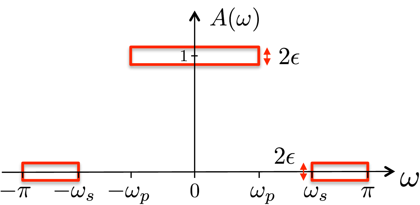
$A(\omega)=h[M/2]~+~ \sum_{n=0}^{M/2-1} 2 \, h[n] \cos(\omega (n-M/2))$Because (generalized) linear phase is desirable, we can focus on meeting filter specifications in terms of modifying $A(\omega)$:
FIR filter design amounts to creating an $A(\omega)$ to fit particular specifications. The goal will be to meet the requirements with as small of a filter size as possible. To that end, there are two pieces of information that will be very useful for us. Both involve the "ripples" of $A(\omega)$ centered around $A(\omega)=1$ in the pass-band and $A(\omega)=0$ in the stop-band. It turns out that among all filters that meet some defined specifications on $A(\omega)$ (the error bounds in the pass- and stop-bands and the pass and stop frequencies), the filter of shortest length $M+1$ will:
--be an
equiripple filter , meaning that all of the ripple oscillations will be of the same deviation about $A(\omega)=1$ in the pass-band and $A(\omega)=0$ in the stop-band (in this sense, the "spread" equally the error out over the entire frequency range)
--will touch theerror bounding box $\frac{M}{2}+2$ times
Putting those properties together, we can see that there are two ways of going about FIR equiripple filter design. One way might be to specify the desired filter length $N=M+1$ (or, equivalently,
filter order $M$), and then use the properties to create an equiripple filter based upon pass-band and stop-band frequencies; because of the first property, this filter will minimize the maximum deviation from $1$ in the pass-band and from $0$ in the stop-band. To design such a filter, one could use the command firpm in MATLAB. Another approach could be to specify these desired deviations, and then go about finding the filter of minimum length that will satisfy these deviations. To do that, one could use the firpmord command in MATLAB.
Equiripple filter of length $n=21$
Suppose we wanted to create a low-pass filter of length $N=21$ (order $M=20$), with a pass-band from $\omega=0$ to $\omega=.3\pi$ and a stop-band from $\omega=.35\pi$ to $\omega=\pi$. Among all possible FIR filters of length $N=21$, an FIR equiripple filter will have the smallest maximum deviation from the optimal frequency response magnitudes (of $|H(\omega)|=1$ in the pass-band and $|H(\omega)|=0$ in the stop-band). According to the equiripple filter properties, its frequency response will touch these error bounding boxes $\frac{M}{2}+2=12$ times.
CAPTION.CAPTION.CAPTION. The equiripple filter is also designed, as described above, to have an impulse response that has even symmetry about its $n=10$ center time value. As a result, it will have a generalized linear phase:
CAPTION.CAPTION.CAPTION. Finally, as this filter is an FIR filter, it will not have any poles (except for those at $z=0$ and, if it were acausal, at $z=\infty$). Since its order is $M=20$, it does have $20$ zeros:
CAPTION.
Equiripple filter of length $n=101$
The filter in the first example, while optimal for its length, still has considerable deviation from the ideal frequency response of $1$ in the pass-band and $0$ in the stop-band. Having a more ideal response is straightforward, simply increase the length of the filter; as described above, the MATLAB command firpmord could be used to tell us the minimum length required to achieve a certain margin of tolerance from the ideal response. Suppose we had some requirement in mind, and that command told us a filter length of $101$ was required. The resulting equiripple filter of that length is below.
CAPTION.CAPTION.CAPTION.CAPTION.