

| << Chapter < Page | Chapter >> Page > |
Now, these two sorting methods achieve the same results, but the Merge Sort typically does so in far fewer steps (although the Bubble Sort will process an already or nearly sorted list quicker). If there are $N$ items in a list, Merge Sort requires about $N\log_2 N$ steps, while the Bubble Sort requires about $N^2$. Even with lists as small as $32$ items, that makes a big difference, the difference between $160$ and $1024$. So it is with the discrete Fourier transform. The DFT is a simple formula: $X[k]=\sum_limits_{n=0}^{N-1}x[n]e^{-j\frac{2\pi}{N}kn}$It would be possible to calculate this as a sum of $N$ multplications (going from $n=0$ to $n=N-1$), doing that $N$ times (for each $k$, again from $0$ to $N-1$). That's about $N^2$ multiplications and additions. But, there are many different ways one could calculate the DFT, just as there are many ways to sort a list. As with Merge Sort, there is a divide-and-conquer approach to finding the DFT which does so with far fewer computational steps, only about $N\log_2 N$.
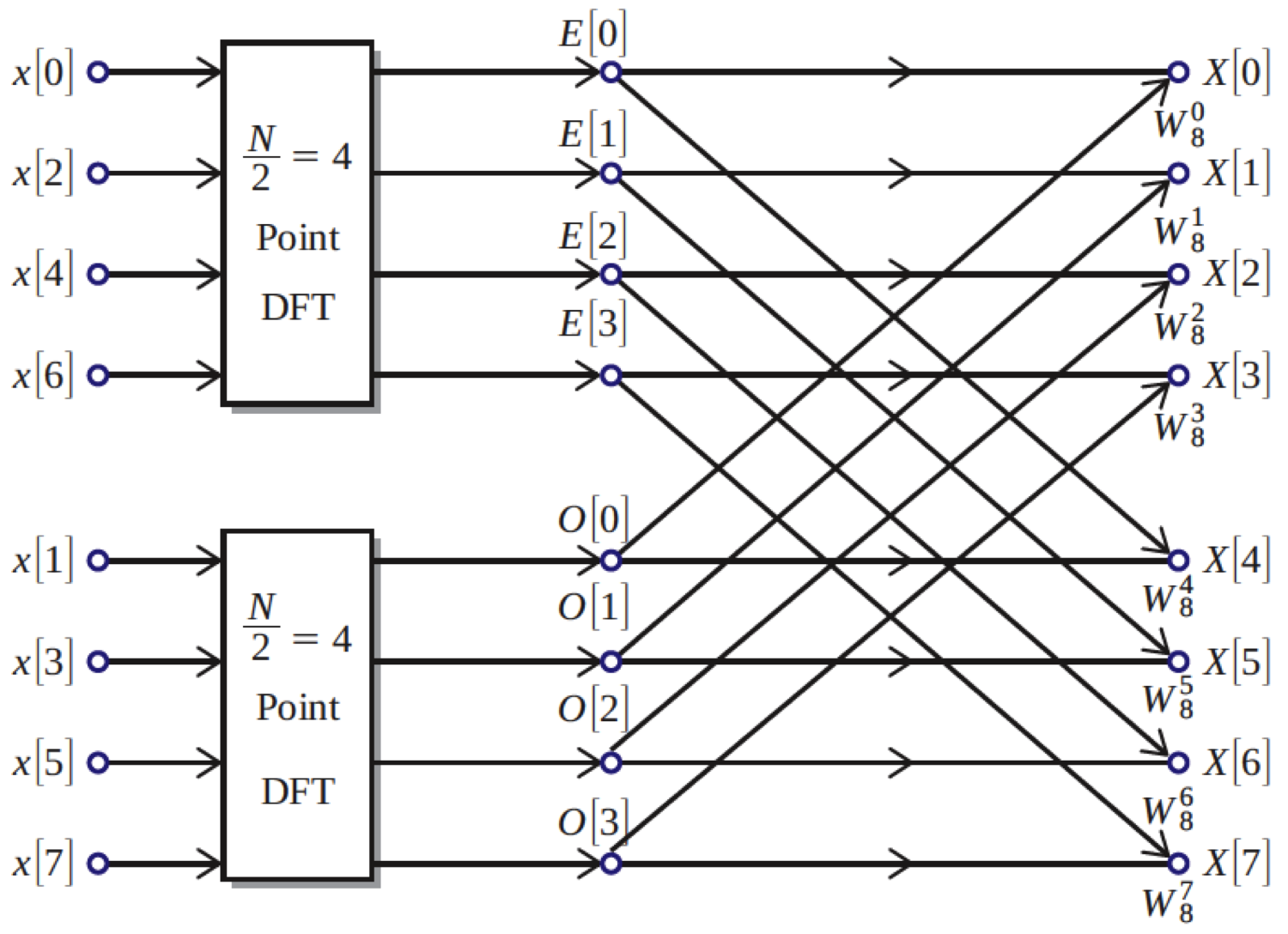
Something similar happens with the DFT. Suppose you have some signal $x[n]$, which you can split into two smaller signals terms of its even and odd indices, $x[2n]$ and $x[2n+1]$. Suppose now that you already know the DFTs of these two smaller signals, and call them $E[k]$ and $O[k]$. Then it is easy to find the DFT of the whole signal, $X[k]$, from these smaller ones: $X[k]=E[k]+e^{j\frac{2\pi}{N}k}O[k]$ A proof of this follows. For simplification of notation, we let $W_N=e^{-j\frac{2\pi}{N}}$:$\begin{align*} X[k]&= \sum_{n=0}^{N-1} x[n]\, W_N^{kn}\\&=\sum_{n=0}^{N/2-1} x[2n]\, W_N^{k (2n)} ~+~\sum_{n=0}^{N/2-1} x[2n+1]\, W_N^{k(2n+1)}\\&=\sum_{n=0}^{N/2-1} x[2n]\, W_N^{2kn} ~+~ W_N^k \sum_{n=0}^{N/2-1} x[2n+1]\, W_N^{2kn} \\&=\sum_{n=0}^{N/2-1} x[2n]\, W_{N/2}^{kn} ~+~ W_N^k \sum_{n=0}^{N/2-1} x[2n+1]\, W_{N/2}^{kn} \\&=E[k] ~+~ W_N^k\, O[k]\end{align*}$ You will note that the $k$ in $X[k]$ runs from $0$ to $N-1$, but that the even and odd DFTs are only of length $N/2$. It seems a little odd, then to consider the values of these DFTs for $k$ greater than $N/2$ (as is necessary in the formula). But there is no problem with this, since DFTs are periodic; as those DFTs are length $N/2$, we have $E[N/2+k]=E[k]$ for those values between $N/2$ and $N-1$. So, we have that the DFT of an $N$-length signal is simply the weigthed sum of 2 $N/2$-length DFTs. And if we, somehow, are given the DFT of those even/odd sub-signals, there are only $N$ additions and multiplications involved in finding the DFT of the whole signal, which is of course much better than the $N^2$ needed to find the DFT by straightforward calculation of the DFT sum.
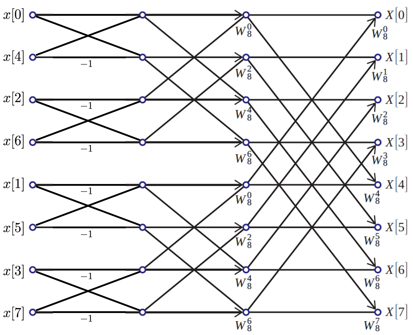
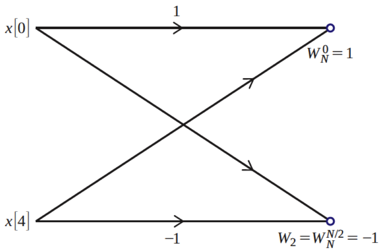
Of course, this requires that we somehow had the DFTs of the sub-divided signals! How do we find those? Well, again we will divide those sub-signals by even/odd indices, and then do that again, and again, until we have lots of length-2 sub-signals. The DFT of a length-2 signal is very easy to compute. If we call such a signal $t[n]$, then $T[0]=t[0]+t[1]$ and $T[1]=t[0]-t[1]$ (this is easy to verify for yourself).
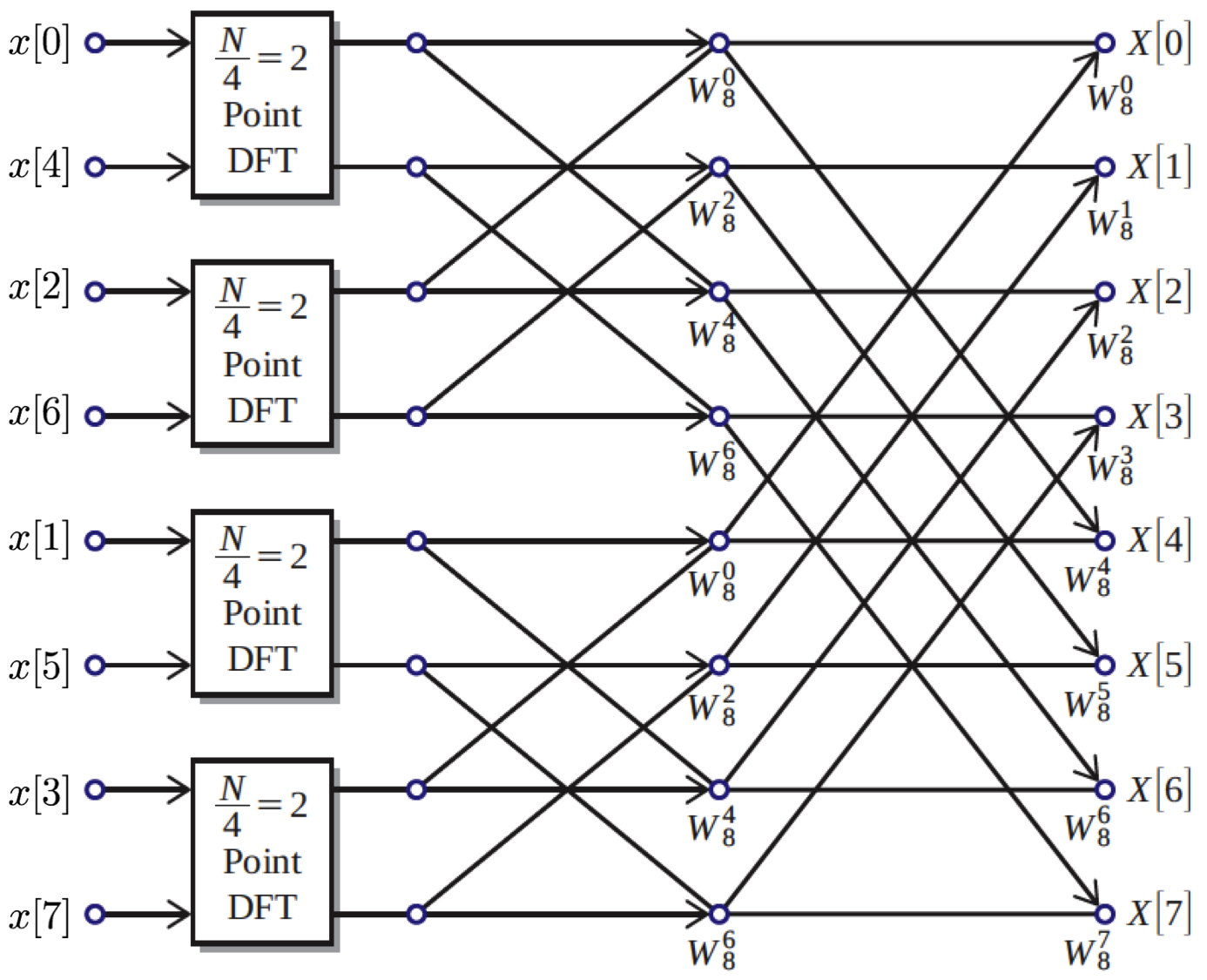
With the DFTs of our many length-2 signals in hand, we use the even/odd sum formula to combine them find the DFT of the length-4 signals, and then length-8, and so on until we have the DFT of the whole signal. This is known as a decimation-in-time FFT, and while it assumes a signal length that is a power of 2, there are ways to apply the approach to signals of other lengths. The figure below illustrates the process of splitting up the DFT into smaller and smaller half-size DFTs:
Notification Switch
Would you like to follow the 'Discrete-time signals and systems' conversation and receive update notifications?

|
|

|
|

|
|

|
|

|
|

|
|

|
|

|
|

|
|

|