Figure 1 Output from the program named Dsp039a
Published: February 22, 2005
By Richard G. Baldwin
Java Programming, Notes # 1487
Introducing convolution
This lesson will show you another approach to digital filtering using Java. This approach is known as convolution. With digital convolution, all operations are performed strictly in the time domain. There is no requirement to transform into the frequency domain.
(The programs in this lesson will transform into the frequency domain, but that will be done solely to show the results of filtering in the time domain.)
Viewing tip
You may find it useful to open another copy of this lesson in a separate browser window. That will make it easier for you to scroll back and forth among the different figures and listings while you are reading about them.
Supplementary material
I recommend that you also study the other lessons in my extensive collection of online Java tutorials. You will find those lessons published at Gamelan.com. However, as of the date of this writing, Gamelan doesn't maintain a consolidated index of my Java tutorial lessons, and sometimes they are difficult to locate there. You will find a consolidated index at www.DickBaldwin.com.
The purpose of this lesson is to help you understand the use of convolution for frequency filtering. A future lesson will explain the use of convolution for matched filtering.
I won't attempt to explain the theoretical basis for convolution. If you search the web using Google, you will undoubtedly find numerous links to theoretical discussions of convolution. Rather, I will explain and illustrate convolution in practical terms.
Computationally, convolution involves sliding one time series along another time series and performing a very simple arithmetic operation at each registration point where the samples in the two time series line up. We can refer to one of the time series as the data and the other as the convolution operator, or simply operator.
Both time series must consist of samples taken at uniform intervals in time, and both must have been sampled at the same sampling rate.
Another example of a sum of products
In several previous lessons, I have explained that one of the most common operations in DSP is to multiply corresponding samples from two time series and to compute the sum of the products. Convolution is no exception to that rule.
In convolution, the operator is matched up against corresponding samples in the data. Then the sum of the products of the corresponding samples is computed. Sometimes that sum is divided by some constant, such as the number of samples in the operator. The sum of the products, possibly divided by a constant, represents one output value.
Then the operator is moved forward by one sample interval, and the sum of products operation is repeated producing another output value.
This process continues, moving the operator forward one sample interval at a time and computing the sum of products of corresponding samples until the operator reaches the end of the data. One output sample is produced during each sum of products operation.
Flip the operator end-for-end
For reasons that I won't go into, the operator must be flipped end-for-end before the process begins. In other words, the sample in the operator that represents the oldest sample in time must be the leading sample as the operator moves along the data.
End effects
As a practical matter, for digital data that has been captured, the data always has a beginning point and an ending point. It is never quite clear how to handle the computational process at the ends.
For example, the process could begin with the operator completely overlapping the data. The process could end at the last point where the operator is completely overlapped with the data. With this approach, the number of output values will always be less than the number of samples in the data (unless the operator has only one sample, which is a trivial case).
Alternatively, the process could begin and/or end at the point where only one sample belonging to the operator overlaps the first and/or last sample in the data. This will produce plenty of output values, but the values computed with less than full overlap are subject to quality concerns.
Probably the best approach is to make certain that you capture enough data that you can afford to sacrifice some output values at the beginning and the end, and to preserve only those output samples computed with a full overlap between the operator and the data.
A practical example
Consider the simple case where the operator consists of two samples each having a value of +1. If you divide the sum of products by two when you convolve this operator with a time series, you are in effect computing a running two-point average of the values in the time series.
(That is to say, each output value is the average of two successive samples in the data. This is not a trivial case, but rather can be useful in some situations.)
Without explaining why, I will tell you that this has the effect of preserving low frequency components and suppressing high-frequency components in the time series.
Another simple-two point operator
If one of the samples in a two-point operator has a value of +1 and the other sample has a value of -1, the results will be completely different. This has the effect of preserving high-frequency components and suppressing low-frequency components.
I will present and explain three programs in this lesson. The first program named Dsp039a creates a convolution operator consisting of a short time series with a linear FM sweep. A Fourier Transform algorithm and a utility plotting program named Graph03 are used to show you the frequency response exhibited by that convolution operator.
(I have explained the use of the Fourier Transform for spectral analysis in several previous lessons, which began with the lesson titled Fun with Java, How and Why Spectral Analysis Works. The previous lesson was titled Fun with Java, Understanding the Fast Fourier Transform (FFT) Algorithm.)
The second program named Dsp039b applies the same convolution operator to a time series consisting of a sequence of equally spaced impulses. The Fourier Transform algorithm and the plotting program are used to show you the spectral content of the time series before and after convolution filtering. In other words, plots show the effect of the convolution operation both in the time domain and in the frequency domain.
The third program named Dsp039c is similar to Dsp039b, except that it applies the convolution filter to white noise and shows you the results in the time domain and in the frequency domain.
The program named Graph03
The program named Graph03 is a utility plotting program from a series of programs first discussed in the lesson titled Plotting Engineering and Scientific Data using Java. I will refer you to that lesson for a detailed discussion of the concepts involved.
A listing of the program is provided in Listing 25 near the end of the lesson. Similarly, a listing of a required interface named GraphIntfc01 is provided in Listing 26 near the end of the lesson.
The program named Dsp039a
As explained earlier, this series of programs illustrates the use of convolution for frequency filtering.
The series consists of the following three programs:
The frequency response of a convolution operator
The program named Dsp039a computes and displays the frequency response of a convolution operator consisting of a pulse with a linear frequency-modulated sweep and constant amplitude across the length of the pulse.
The frequency modulation sweeps from 1000 HZ to 2000 HZ at an assumed sampling rate of 16000 samples per second.
(If a different sampling rate is assumed, the boundary frequencies at the ends of the sweep will also be different.)
The program output
The top plot in Figure 1 shows the convolution operator. The bottom plot in Figure 1 shows the frequency response of that operator.
|
Running the program
You can run this program by entering the following command at the command-line prompt.
java Graph03 Dsp039a
When run in this manner, the program requires access to the following program files, all of which are provided near the end of the lesson:
The program was tested using JDK 1.4.2 under WinXP.
Discussion of the code for Dsp039a
The class definition for Dsp039a begins in Listing 1. Note that this class implements GraphIntfc01. This is necessary to satisfy the requirements of the utility plotting program named Graph03.
class Dsp039a implements GraphIntfc01{
  int operLen = 50;
  int windowLen = 400;
  int spectrumPts = windowLen - operLen;

Listing 1
|
The code in Listing 1 establishes:
(The value specified for the number of spectral points may look a little strange at this point. This value was chosen to be consistent with spectral analyses that will be performed in the other two programs discussed later in this lesson.)
Create the arrays
The code in Listing 2 creates the arrays that will be used to store the window, the operator, and the frequency response of the operator.
double[] window = new double[windowLen]; double[] operator = new double[operLen]; double[] spectrumA = new double[spectrumPts]; Listing 2 |
The constructor
The constructor begins in Listing 3.
  public Dsp039a(){//constructor

    fmSweep(operLen,operator);

Listing 3
|
The code in Listing 3 invokes a method named fmSweep, which returns a time series that will be used as a convolution operator.
The method named fmSweep
I will set the discussion of the constructor aside for a moment and discuss the method named fmSweep.
As mentioned earlier, the top plot in Figure 1 shows the waveform of the time series produced by this method.
As you can see from Figure 1, the waveform is sort of sinusoidal with the period decreasing, or the frequency increasing as you move from left to right across the pulse.
(The fact that each of the peaks doesn't appear to be the same height is an artifact of the sampling process. As you move to the right, some of the peaks fall in between samples.)
The code for the fmSweep method
This method generates a pulse with a linear frequency sweep from 1000 Hz to 2000 Hz at an assumed sampling rate of 16000 samples per second.
The code in Listing 4 declares and initializes some local variables. The names of these variables should be sufficient to indicate their purpose.
  void fmSweep(int pulseLen,double[] output){
    double twoPI = 2*Math.PI;
    double sampleRate = 16000.0;
    double lowFreq = 1000.0;
    double highFreq = 2000.0;

Listing 4
|
Incoming parameters
The first parameter to the fmSweep method specifies the length of the desired pulse in samples.
The second parameter is a reference to an array of type double where the method is to deposit the output.
Populate the output array
The code in Listing 5 computes the samples and stores them in the output array.
    for(int cnt = 0; cnt < pulseLen; cnt++){
      double time = cnt/sampleRate;

      double freq = lowFreq +
                 cnt*(highFreq-lowFreq)/pulseLen;
      double sinValue =
                       Math.sin(twoPI*freq*time);
      output[cnt] = sinValue;
    }//end for loop
  }//end method fmSweep

Listing 5
|
Now that you know what to look for, the code in Listing 5 shouldn't require a detailed explanation. Once again, the sample values produced by this method are displayed in the top plot in Figure 1.
Back to the constructor
Returning now to the discussion of the constructor, the code in Listing 6 adds the convolution operator to a longer time series consisting of all zero values.
    for(int cnt = 0; cnt < operLen; cnt++){
      window[cnt] += operator[cnt];
    }//end for loop

Listing 6
|
This is done as a convenience for spectrum analysis. This makes it possible to use an existing DFT algorithm, which computes the spectrum at a number of points equal to the length of the data. This, in turn, causes the spectrum to be computed at a sufficient number of points to produce a smooth spectral estimate. It also causes the plot of the spectral estimate to be consistent with spectral plots produced by other programs in this lesson.
The code in Listing 6 is straightforward and shouldn't require further explanation.
Compute the frequency response
The code in Listing 7 invokes a Discrete Fourier Transform (DFT) method to compute the frequency response of the convolution operator.
    Dft01.dft(window,spectrumPts,spectrumA);

Listing 7
|
The dft method receives references to two arrays and an integer value:
Several previous lessons, including the lesson titled Spectrum Analysis using Java, Sampling Frequency, Folding Frequency, and the FFT Algorithm, have discussed spectral analysis in detail. Therefore, I won't discuss the method named dft in this lesson. You will find it in Listing 22 near the end of the lesson.
The output produced by the dft method is shown as the bottom plot in Figure 1.
End of the constructor
Listing 7 also signals the end of the constructor.
Graphic support methods
At this point, all of the data that is to be plotted for Dsp039a has been computed and saved in arrays.
In order to be compatible with the plotting program named Graph03, this class implements the interface named GraphIntfc01. That interface declares six methods named:
Plotting from one to five curves
Referring back to Figure 1, you can see that two different curves were plotted in Figure 1. The top curve is the convolution operator that I discussed earlier. The bottom curve is the frequency response of the convolution operator that I will discuss shortly.
The program named Graph03 can plot from one to five curves in the same frame. The program invokes the method named getNmbr to determine how many curves to plot. In this program, the getNmbr method returned a value of 2, indicating that two curves should be plotted.
Getting the data to be plotted
Each of the methods named f1 through f5 supplies the data to be plotted in one of the five plots.
(For fewer than five plots, the methods having higher numbers in their names aren't called. Once again, you can read about these concepts in the lesson titled Plotting Engineering and Scientific Data using Java.)
For each curve that is to be plotted for this program, the Graph03 method calls the methods named f1 or f2 repeatedly. Each time one of these method is called, it returns the next value that is to be plotted.
The six interface methods
The implementation of each of the six interface methods is shown in Listing 8.
  //The following six methods are required by the
  // interface named GraphIntfc01.
  public int getNmbr(){
    //Return number of functions to process. Must
    // not exceed 5.
    //A return value of 2 causes two curves to be
    // plotted and also causes the last three of
    // the following five methods to be ignored
    // by the plotting program.
    return 2;
  }//end getNmbr
  //-------------------------------------------//

  public double f1(double x){
    int index = (int)Math.round(x);
    //Return the convolution operator added to a
    // time series with all sample values equal
    // to zero.
    if(index < 0 || index > window.length-1){
      return 0;
    }else{
      //Scale for display and return.
      return window[index] * 50.0;
    }//end else
  }//end f1
  //-------------------------------------------//

  public double f2(double x){
    //Return the spectral response of the
    // convolution operator.
    int index = (int)Math.round(x);
    if(index < 0 || index > spectrumA.length-1){
      return 0;
    }else{
      //Scale for display and return.
      return spectrumA[index] * 7.0;
    }//end else
  }//end f2
  //-------------------------------------------//

  public double f3(double x){
    return 0.0;
  }//end f3
  //-------------------------------------------//

  public double f4(double x){
    return 0.0;
  }//end f4
  //-------------------------------------------//

  public double f5(double x){
    return 0.0;
  }//end f5

Listing 8
|
The general discussion above along with the comments in Listing 8 should suffice, and it should not be necessary for me to discuss these methods further in this lesson.
Scaling the data for plotting
It is important to note, however, that the methods named f1 and f2 apply a scale factor to the data samples before returning them.
(This will also be true of the methods named f3, f4, and f5 in the remaining two programs in this lesson.)
The purpose of the scale factor is to cause all of the plots in the frame to have approximately the same range. Otherwise, some plots would be too large to fit in the allowable space while others would be so small as to make it impossible to see any detail.
The frequency response of the convolution operator
Now please turn your attention to the bottom plot in Figure 1. This is a plot of the frequency response of the convolution filter shown in the top plot.
What do I mean by frequency response?
If a time series is filtered by convolving it with this operator, the spectral content of the filtered time series will be the product of the original spectral content of the time series and the spectral content shown by the bottom plot in Figure 1.
Format of Figure 1
The bottom plot in Figure 1 shows the spectral content of the convolution operator from a frequency of zero on the left to a frequency equal to the sampling frequency about half way between the seventeenth and eighteenth tick marks on the right.
The Nyquist folding frequency
The Nyquist folding frequency occurs at a point in the plot that is half the sampling frequency.
(See the lesson titled Spectrum Analysis using Java, Sampling Frequency, Folding Frequency, and the FFT Algorithm for a detailed discussion of the Nyquist folding frequency.)
Spectral values above the folding frequency are a mirror image of the values below the folding frequency. Therefore, you can concentrate on those values below the folding frequency and ignore the values above the folding frequency.
Discussion of the frequency response
As you can see, frequencies between the third tick mark and the folding frequency will be strongly suppressed because the response is near zero at these frequencies.
(When the spectral content values of a time series are multiplied by these values, the result will be near zero.)
Similarly, frequencies below the first tick mark will also be suppressed for the same reason.
Frequencies closely surrounding the second tick mark will be preserved because the response of the convolution operator at these frequencies is high.
We will see examples of the suppression of some frequency components and the preservation of other frequency components later when we apply this convolution operator to time series having strong frequency components all the way from zero to the folding frequency.
The program named Dsp039b
As you have just learned, the program named Dsp039a illustrates the frequency response of a particular convolution filter.
The program named Dsp039b illustrates the result of applying that convolution filter to a time series consisting of a series of equally spaced impulses.
Dsp039c, which I will discuss later, illustrates the result of applying the same convolution filter to a time series consisting of white noise.
Running the program
You can run this program by entering the following command at the command-line prompt:
java Graph03 Dsp039b
The program was tested using JDK 1.4.2 under WinXP.
The program output
This program, in combination with the program named Graph03, displays five different plots as shown in Figure 2.
|
Proceeding from top to bottom, the five plots shown in Figure 2 are:
The bottom line
Compare the bottom two plots in Figure 2. Imagine the spectral values for the raw data plot being multiplied by the frequency response of the convolution operator shown in Figure 1.
As described earlier, frequency components near the second tick mark are preserved in the output spectrum in the bottom plot in Figure 2. Frequency components below the first tick mark and frequency components above the third tick mark are strongly suppressed.
Discussion of the code for Dsp039b
The class definition for Dsp039b begins in Listing 9.
class Dsp039b implements GraphIntfc01{
  int operLen = 50;
  int dataLen = 400;
  int outputLen = dataLen - operLen;
  int spectrumPts = outputLen;

Listing 9
|
This program begins in a way that is very similar to the previous program. Listing 9 declares and initializes some instance variables. The values stored in these variables will be used later.
Create the arrays
Listing 10 creates several empty arrays. These arrays will be used for intermediate data storage, and to save the program output for plotting.
double[] data = new double[dataLen]; double[] operator = new double[operLen]; double[] output = new double[outputLen]; double[] spectrumA = new double[spectrumPts]; double[] spectrumB = new double[spectrumPts]; Listing 10 |
Generate the input data
The constructor begins in Listing 11.
  public Dsp039b(){//constructor

    for(int cnt = 0;cnt < dataLen;cnt++){
      if(cnt%25 == 0)data[cnt] = 1;
    }//end for loop

Listing 11
|
Listing 11 generates and saves an input time series consisting of a series of equally spaced impulses. Every twenty-fifth sample in the time series has a value of one. All other samples have a value of zero.
This time series is shown in the top plot of Figure 2.
The convolution operator
Listing 12 creates and saves the same convolution operator that was discussed in the previous program named Dsp039a.
    fmSweep(operLen,operator);

Listing 12
|
The convolution operator is shown in the second plot in Figure 2.
Perform the convolution
Listing 13 applies the convolution operator to the data causing the result of the convolution to be saved in the array referred to by output.
    Convolve01.convolve(data,operator,output);

Listing 13
|
The method named convolve
At this point, I will set the discussion of the constructor aside temporarily and explain the method named convolve.
Listing 14 shows the beginning of a class named Convolve01.
class Convolve01{
  public static void convolve(double[] data,
                              double[] operator,
                              double[] output){


Listing 14
|
The Convolve01 class provides a static method named convolve, which applies an incoming convolution operator to an incoming set of data, and deposits the filtered result in an output array whose reference is received as an incoming parameter.
The convolution loop
Listing 15 applies the convolution operator to the data, dealing with the requirement to flip the convolution operator end-for-end.
    int dataLen = data.length;
    int operatorLen = operator.length;

    for(int i = 0;i < dataLen-operatorLen;i++){
      output[i] = 0;
      for(int j = operatorLen-1;j >= 0;j--){
        output[i] += data[i+j]*operator[j];
      }//end inner loop
    }//end outer loop
  }//end convolve method
}//end Class Convolve01

Listing 15
|
Please refer back to the section in this lesson titled "What is convolution?" as you examine the code in Listing 15.
You should be able to see how the code in Listing 15 slides the convolution operator across the data, progressing one sample interval at a time, and computing the sum of products for each registration of convolution samples and data samples.
The convolution output
The output time series produced by the convolution operation is shown in the third plot in Figure 2. This plot shows the result of filtering the input data in the first plot with the convolution operator in the second plot.
Compute the raw data spectrum
Returning now to the constructor, the code in Listing 16 uses the dft method discussed earlier to compute the spectrum of the raw data.
    Dft01.dft(data,spectrumPts,spectrumA);

Listing 16
|
The spectral estimate for the raw data is saved in the array referred to by spectrumA, and is plotted in the fourth plot in Figure 2.
As you can see, the spectral content of the series of equally spaced impulses in the time domain is a series of equally spaced frequency components each having equal strength.
Compute the filtered data spectrum
Listing 17 invokes the dft method to estimate the spectral content of the filtered data and saves the results in an array referred to by spectrumB.
    Dft01.dft(output,spectrumPts,spectrumB);

Listing 17
|
The spectral estimate of the filtered data is shown in the bottom plot in Figure 2.
As discussed earlier, the spectral content of the filtered data is given by the product of the spectral content of the raw data and the frequency response of the convolution operator shown in Figure 1.
Frequency components at and surrounding the second tick mark are preserved, while frequency components below the first tick mark and above the third tick mark are suppressed.
The interface methods
The six interface methods, which specify the number of plots, and return the data for plotting, are shown in Listing 18.
  //The following six methods are required by the
  // interface named GraphIntfc01.
  public int getNmbr(){
    //Return number of functions to process. Must
    // not exceed 5.
    return 5;
  }//end getNmbr
  //-------------------------------------------//

  public double f1(double x){
    int index = (int)Math.round(x);
    //This method returns the raw data values.
    if(index < 0 || index > data.length-1){
      return 0;
    }else{
      //Scale for display and return.
      return data[index] * 90.0;
    }//end else
  }//end f1
  //-------------------------------------------//

  public double f2(double x){
    //Return the convolution operator
    int index = (int)Math.round(x);
    if(index < 0 || index > operator.length-1){
      return 0;
    }else{
      //Scale for display and return.
      return operator[index] * 90.0;
    }//end else
  }//end f2
  //-------------------------------------------//

  public double f3(double x){
    //Return convolution output
    int index = (int)Math.round(x);
    if(index < 0 || index > output.length-1){
      return 0;
    }else{
      //Scale for display and return.
      return output[index] * 50.0;
    }//end else
  }//end f3
  //-------------------------------------------//

  public double f4(double x){
    //Return spectrum of the raw data
    int index = (int)Math.round(x);
    if(index < 0 || index > spectrumA.length-1){
      return 0;
    }else{
      //Scale for display and return.
      return spectrumA[index] * 5.0;
    }//end else
  }//end f4
  //-------------------------------------------//

  public double f5(double x){
    //Return the spectrum of the filtered data
    int index = (int)Math.round(x);
    if(index < 0 || index > spectrumB.length-1){
      return 0;
    }else{
      //Scale for display and return.
      return spectrumB[index]*0.60;
    }//end else
  }//end f5

Listing 18
|
These methods are straightforward and won't be discussed further.
The fmSweep and dft methods
The methods named fmSweep and dft are identical to the methods having the same name used in the program named Dsp039a. These methods can be viewed in Listing 23 near the end of the lesson.
The program named Dsp039c
The program named Dsp039a illustrates the frequency response of a convolution filter.
The program named Dsp039b illustrates the result of applying that convolution filter to a time series consisting of a series of equally spaced impulses.
This program, named Dsp039c illustrates the result of applying that same convolution filter to a time series consisting of white noise.
What is white noise?
The term white noise comes from the term white light. Theoretically, white light, as emitted by the sun, contains an equal distribution of energy at all wavelengths in the visible spectrum. If you apply an optical filter such as a piece of translucent red glass, much of the energy will be removed, leaving only the wavelengths in the red end of the spectrum.
The term white noise applies to noise that theoretically contains an equal distribution of energy at all frequencies. A good approximation of white noise in the world of sampled data is a series of values taken from a random number generator.
The reality of short samples
In reality, no finite length sample of random numbers contains an equal distribution of energy at all frequencies between zero and the folding frequency.
The spectral content of one series of random numbers will exhibit one shape, and the spectral content of another series of random numbers will exhibit a different shape.
(On average, the spectral content of a large number of such series of random numbers will approximate an equal distribution of energy at all frequencies between zero and the folding frequency.)
The longer the sample, however, the closer will be the approximation to an equal distribution of energy at all frequencies between zero and the folding frequency.
When you run this program, you will see the spectral content of a series of 400 random numbers. Each time you run the program, you will see the spectral content of a different series of 400 random numbers taken from the same random number generator.
Running the program
You can run this program by entering the following command at the command-line prompt:
java Graph03 Dsp039c
This program was tested using JDK 1.4.2 under WinXP.
The program output
The program output for one such run is shown in Figure 3.
|
Going from top to bottom, the five plots show:
The bottom line
If you compare the filtered output in the third plot with the raw data in the first plot, you can see that the filtered output is richer in terms of low-frequency components. This is consistent with the frequency response of the convolution operator shown in Figure 1. That filter tends to preserve low-frequency components and to suppress high-frequency components.
Also, if you compare the bottom two plots in Figure 3, you can imagine that the shape of the bottom plot is an approximation of the product of the spectral content of the raw data and the frequency response of the convolution operator shown in Figure 1.
Since the frequency response is not flat, the spectral content in the area of the second tick mark doesn't look exactly like the spectral content of the raw data in that same area. However, as before, the energy was preserved in the area surrounding the second tick mark. Energy below the first tick mark and energy above the third tick mark was suppressed.
Discussion of the code for Dsp039c
The class definition for Dsp039c begins in Listing 19.
class Dsp039c implements GraphIntfc01{
  //Establish length for operator, data, and
  // spectrum
  int operLen = 50;
  int dataLen = 400;
  int outputLen = dataLen - operLen;
  int spectrumPts = outputLen;

  //Create arrays for the data and the results.
  double[] data = new double[dataLen];
  double[] operator = new double[operLen];
  double[] output = new double[outputLen];

  double[] spectrumA = new double[spectrumPts];
  double[] spectrumB = new double[spectrumPts];

Listing 19
|
This program is very similar to the program named Dsp039b. The only real difference has to do with the source of the raw data.
The code in Listing 19 is essentially the same as the code presented earlier in Listings 10 and 11.
Generate the white noise
The constructor begins in Listing 20.
  public Dsp039c(){//constructor

    Random generator = new Random(
                           new Date().getTime());

    for(int cnt=0;cnt < data.length;cnt++){
      data[cnt] =
              2.0*(generator.nextDouble() - 0.5);
    }//end for loop

Listing 20
|
Listing 20 contains the code to use a random number generator to get and save 400 random numbers. I will refer you to the Sun documentation and the class named Random if you need to know more about using that class to get random numbers.
A different seed for each run
The random number generator uses a seed as input when it generates the set of random numbers. If two or more sets of random numbers are generated using the same seed, the values of the random numbers will be the same.
If two or more sets of random numbers are generated using different seeds, the values in the two sets of numbers will be different, and the numbers will be random with respect to one another.
(This implies that the cross-correlation between the two sets of values is very low, but cross-correlation is a DSP topic for a different lesson.)
Use the time as a seed
Listing 20 gets the date and time in milliseconds, relative to January 1, 1970, and uses that value as a seed each time the program is run. Therefore, unless it is possible to run the program twice within one millisecond, there is no way that two different runs of the program can produce the same set of random numbers.
Eliminate the bias and scale the value
Each random number produced by the method named nextDouble in Listing 20 has a value uniformly distributed between 0 and 1.0. Hence, the average value of the random numbers is 0.5.
The code in Listing 20 subtracts 0.5 from each random number to cause the values to be distributed between negative 0.5 and positive 0.5. Then those values are multiplied by 2.0 to cause the values to be distributed between negative 1.0 and positive 1.0. This is what you see in the first plot in Figure 3 (except that each value has been multiplied by 50.0 in method f1 to bring it into a good plotting range).
The remaining code
The remaining code in the constructor is shown in Listing 21.
    //Create a convolution operator.
    fmSweep(operLen,operator);

    //Apply the convolution operator to the white
    // noise.
    Convolve01.convolve(data,operator,output);

    //Compute DFT of the raw white noise. Save it
    // in spectrumA array.
    Dft01.dft(data,spectrumPts,spectrumA);

    //Compute DFT of the filtered white noise and
    // save it in spectrumB array.
    Dft01.dft(output,spectrumPts,
                            spectrumB);

  }//end constructor

Listing 21
|
The code in Listing 21 accomplishes the following:
This code is essentially the same as the code discussed in conjunction with the program named Dsp039b, so I won't discuss it further here.
The six interface methods
The implementation of the six interface methods in the program named Dsp039c is shown in Listing 22.
  //The following six methods are required by the
  // interface named GraphIntfc01.
  public int getNmbr(){
    //Return number of functions to process. Must
    // not exceed 5.
    return 5;
  }//end getNmbr
  //-------------------------------------------//
  public double f1(double x){
    int index = (int)Math.round(x);
    //This method returns the raw white noise.
    if(index < 0 || index > data.length-1){
      return 0;
    }else{
      //Scale for display and return.
      return data[index] * 50.0;
    }//end else
  }//end f1
  //-------------------------------------------//
  public double f2(double x){
    //Return the convolution operator
    int index = (int)Math.round(x);
    if(index < 0 || index > operator.length-1){
      return 0;
    }else{
      //Scale for display and return.
      return operator[index] * 50.0;
    }//end else
  }//end f2
  //-------------------------------------------//
  public double f3(double x){
    //Return the filtered noise
    int index = (int)Math.round(x);
    if(index < 0 || index > output.length-1){
      return 0;
    }else{
      //Scale for display and return.
      return output[index] * 7.0;
    }//end else
  }//end f3
  //-------------------------------------------//
  public double f4(double x){
    //Return spectrum of raw white noise
    int index = (int)Math.round(x);
    if(index < 0 || index > spectrumA.length-1){
      return 0;
    }else{
      //Scale for display and return.
      return spectrumA[index] * 4.0;
    }//end else
  }//end f4
  //-------------------------------------------//
  public double f5(double x){
    //Return the spectrum of the filtered white
    // noise.
    int index = (int)Math.round(x);
    if(index < 0 || index > spectrumB.length-1){
      return 0;
    }else{
      //Scale for display and return.
      return spectrumB[index]*0.4;
    }//end else
  }//end f5

Listing 22
|
With the exception of the need for different scale factors to adjust the values for plotting, the methods in Listing 22 are the same as the methods having the same names in Listing 18. Therefore, I won't discuss them further.
The fmSweep, convolve, and dft methods
These methods are identical to the methods having the same names in the program named Dsp039b. Therefore, I won't discuss them further. You can view these methods in Listing 24 near the end of the lesson.
I encourage you to copy, compile, and run the programs that you will find in the listings near the end of the lesson. Modify them and experiment with them in order to learn as much as you can about the use of convolution for frequency filtering.
For example, you might want to create and use different convolution operators, such as the two-point operators discussed earlier in the lesson.
In the next lesson, I will explain and illustrate the use of convolution for a significantly different purpose known commonly as matched filtering.
A complete listing of each of the programs is provided in below.
/* File Dsp039a.java
Copyright 2005, R.G.Baldwin

This series of programs illustrates the use of
convolution for frequency filtering.

The series consists of the following three
programs:

Dsp039a
Dsp039b
Dsp039c

A future program will illustrate the use of
convolution for matched filtering.

This program computes and displays the response
of a convolution operator consisting of a pulse
with a linear frequency-modulated sweep and
constant amplitude across the length of the
pulse.

The frequency modulation sweeps from 1000 HZ to
2000 HZ at an assumed sampling rate of 16000
samples per second.

Dsp039b illustrates the result of applying the
convolution filter to a time series consisting of
a series of equally-spaced impulses.

Dsp039c illustrates the result of applying the
convolution filter to a time series consisting of
white noise.

Run this program by entering the following
command at the command-line prompt.

java Graph03 Dsp039a

When run in this manner, the program requires
access to the following program files:

Graph03.java
GraphIntfc01

Tested using JDK 1.4.2 under WinXP.
************************************************/
import java.util.*;

class Dsp039a implements GraphIntfc01{
  //Establish length for operator, window, and
  // spectrum
  int operLen = 50;
  int windowLen = 400;
  //Compute the spectrum at the number of points
  // defined in the following variable so that
  // the spectral plot will beconsistent with the
  // spectral plots produced by other programs in
  // this series.
  int spectrumPts = windowLen - operLen;

  //Create arrays for the window, the convolution
  // operator, and the spectrum
  double[] window = new double[windowLen];
  double[] operator = new double[operLen];
  double[] spectrumA = new double[spectrumPts];

  public Dsp039a(){//constructor

    //Create and save a convolution operator
    // consisting of a linear FM pulse.
    fmSweep(operLen,operator);

    //Add the convolution operator to a time
    // series consisting of all zero values.
    // This is done as a convenience for spectrum
    // analysis.  This makes it possible to use
    // an existing DFT algorithm that computes
    // the spectrum at a number of points equal
    // to the length of the data. This, in turn,
    // causes the spectrum to be computed at a
    // sufficient number of points to produce a
    // smooth spectral estimate.  It also causes
    // the plot of the spectral estimate to be
    // consistent with spectral plots produced
    // by other programs in this series.
    for(int cnt = 0; cnt < operLen; cnt++){
      window[cnt] += operator[cnt];
    }//end for loop

    //Compute the frequency response of the
    // convolution operator.
    Dft01.dft(window,spectrumPts,spectrumA);

    //All of the time series have now been
    // produced and saved.  They may be
    // retrieved and plotted by invoking the
    // methods named f1 and f2.

  }//end constructor

  //-------------------------------------------//
  //The following six methods are required by the
  // interface named GraphIntfc01.
  public int getNmbr(){
    //Return number of functions to process. Must
    // not exceed 5.
    //A return value of 2 causes two curves to be
    // plotted and also causes the last three of
    // the following five methods to be ignored
    // by the plotting program.
    return 2;
  }//end getNmbr
  //-------------------------------------------//
  public double f1(double x){
    int index = (int)Math.round(x);
    //Return the convolution operator added to a
    // time series with all sample values equal
    // to zero.
    if(index < 0 || index > window.length-1){
      return 0;
    }else{
      //Scale for display and return.
      return window[index] * 50.0;
    }//end else
  }//end f1
  //-------------------------------------------//
  public double f2(double x){
    //Return the spectral response of the
    // convolution operator.
    int index = (int)Math.round(x);
    if(index < 0 || index > spectrumA.length-1){
      return 0;
    }else{
      //Scale for display and return.
      return spectrumA[index] * 7.0;
    }//end else
  }//end f2
  //-------------------------------------------//
  public double f3(double x){
    return 0.0;
  }//end f3
  //-------------------------------------------//
  public double f4(double x){
    return 0.0;
  }//end f4
  //-------------------------------------------//
  public double f5(double x){
    return 0.0;
  }//end f5
  //-------------------------------------------//

  //This method generates a pulse with a linear
  // frequency sweep from 1000 Hz to 2000 Hz at
  // a sampling rate of 16000 samples per
  // second.
  void fmSweep(int pulseLen,double[] output){
    double twoPI = 2*Math.PI;
    double sampleRate = 16000.0;
    double lowFreq = 1000.0;
    double highFreq = 2000.0;

    for(int cnt = 0; cnt < pulseLen; cnt++){
      double time = cnt/sampleRate;

      double freq = lowFreq +
                 cnt*(highFreq-lowFreq)/pulseLen;
      double sinValue =
                       Math.sin(twoPI*freq*time);
      output[cnt] = sinValue;
    }//end for loop
  }//end method fmSweep

}//end class Dsp039a
//=============================================//

//This class provides a static method named dft,
// which computes and returns the amplitude
// spectrum of an incoming time series.  The
// amplitude spectrum is computed as the square
// root of the sum of the squares of the real and
// imaginary parts.
//Returns a number of points in the frequency
// domain equal to the number of samples in the
// incoming time series.  This is for convenience
// only and is not a requirement of a DFT.
//Deposits the frequency data in an array whose
// reference is received as an incoming
// parameter.
class Dft01{
  public static void dft(double[] data,
                         int dataLen,
                         double[] spectrum){
    double twoPI = 2*Math.PI;

    //Set the frequency increment to the
    // reciprocal of the data length.  This is
    // convenience only, and is not a requirement
    // of the DFT algorithm.
    double delF = 1.0/dataLen;
    //Outer loop iterates on frequency values.
    for(int i = 0; i < dataLen;i++){
      double freq = i*delF;
      double real = 0;
      double imag = 0;
      //Inner loop iterates on time- series
      // points.
      for(int j=0; j < dataLen; j++){
        real += data[j]*Math.cos(twoPI*freq*j);
        imag += data[j]*Math.sin(twoPI*freq*j);
        spectrum[i] = Math.sqrt(
                          real*real + imag*imag);
      }//end inner loop
    }//end outer loop
  }//end dft

}//end Dft01

Listing 22
|
/* File Dsp039b.java
Copyright 2005, R.G.Baldwin

This series of programs illustrates the use of
convolution for frequency filtering.

The series consists of the following three
programs:

Dsp039a
Dsp039b
Dsp039c

A future program will illustrate the use of
convolution for matched filtering.

Dsp039a illustrates the frequency response of a
convolution filter.

This  program shows the result of applying that
convolution filter to a time series consisting
of a series of equally-spaced impulses.

Dsp039c illustrates the result of applying the
convolution filter to a time series consisting of
white noise.

Run this program by entering the following
command at the command-line prompt:

java Graph03 Dsp039b

Tested using JDK 1.4.2 under WinXP.
************************************************/
import java.util.*;

class Dsp039b implements GraphIntfc01{
  //Establish length for operator, data, and
  // spectrum
  int operLen = 50;
  int dataLen = 400;
  int outputLen = dataLen - operLen;
  int spectrumPts = outputLen;

  //Create arrays for the data and the results.
  double[] data = new double[dataLen];
  double[] operator = new double[operLen];
  double[] output = new double[outputLen];

  double[] spectrumA = new double[spectrumPts];
  double[] spectrumB = new double[spectrumPts];

  public Dsp039b(){//constructor

    //Generate some wide-band data consisting of
    // a series of equally-spaced impulses
    for(int cnt = 0;cnt < dataLen;cnt++){
      if(cnt%25 == 0)data[cnt] = 1;
    }//end for loop

    //Create and save a convolution operator
    fmSweep(operLen,operator);

    //Apply the convolution operator to the data.
    Convolve01.convolve(data,operator,output);

    //Compute DFT of raw data and  save it in
    // spectrumA array.
    Dft01.dft(data,spectrumPts,spectrumA);

    //Compute DFT of the filtered data and save
    // it in spectrumB array.
    Dft01.dft(output,spectrumPts,spectrumB);

    //All of the time series have now been
    // produced and saved.  They may be
    // retrieved and plotted by invoking the
    // methods named f1 through f5.

  }//end constructor

  //-------------------------------------------//
  //The following six methods are required by the
  // interface named GraphIntfc01.
  public int getNmbr(){
    //Return number of functions to process. Must
    // not exceed 5.
    return 5;
  }//end getNmbr
  //-------------------------------------------//
  public double f1(double x){
    int index = (int)Math.round(x);
    //This method returns the raw data values.
    if(index < 0 || index > data.length-1){
      return 0;
    }else{
      //Scale for display and return.
      return data[index] * 90.0;
    }//end else
  }//end f1
  //-------------------------------------------//
  public double f2(double x){
    //Return the convolution operator
    int index = (int)Math.round(x);
    if(index < 0 || index > operator.length-1){
      return 0;
    }else{
      //Scale for display and return.
      return operator[index] * 90.0;
    }//end else
  }//end f2
  //-------------------------------------------//
  public double f3(double x){
    //Return convolution output
    int index = (int)Math.round(x);
    if(index < 0 || index > output.length-1){
      return 0;
    }else{
      //Scale for display and return.
      return output[index] * 50.0;
    }//end else
  }//end f3
  //-------------------------------------------//
  public double f4(double x){
    //Return spectrum of the raw data
    int index = (int)Math.round(x);
    if(index < 0 || index > spectrumA.length-1){
      return 0;
    }else{
      //Scale for display and return.
      return spectrumA[index] * 5.0;
    }//end else
  }//end f4
  //-------------------------------------------//
  public double f5(double x){
    //Return the spectrum of the filtered data
    int index = (int)Math.round(x);
    if(index < 0 || index > spectrumB.length-1){
      return 0;
    }else{
      //Scale for display and return.
      return spectrumB[index]*0.60;
    }//end else
  }//end f5
  //-------------------------------------------//

  //This method generates a pulse with a linear
  // frequency sweep from 1000 Hz to 2000Hz at
  // a sampling rate of 16000 samples per
  // second.
  void fmSweep(int pulseLen,double[] output){
    double twoPI = 2*Math.PI;
    double sampleRate = 16000.0;
    double lowFreq = 1000.0;
    double highFreq = 2000.0;

    for(int cnt = 0; cnt < pulseLen; cnt++){
      double time = cnt/sampleRate;

      double freq = lowFreq +
                 cnt*(highFreq-lowFreq)/pulseLen;
      double sinValue =
                       Math.sin(twoPI*freq*time);
      output[cnt] = sinValue;
    }//end for loop
  }//end method fmSweep

}//end class Dsp039b
//=============================================//

//This class provides a static method named
// convolve, which applies an incoming
// convolution operator to an incoming set of
// data and deposits the filtered data in an
// output array whose reference is received as an
// incoming parameter.
class Convolve01{
  public static void convolve(double[] data,
                              double[] operator,
                              double[] output){
    //Apply the operator to the data, dealing
    // with the index reversal required by
    // convolution.
    int dataLen = data.length;
    int operatorLen = operator.length;
    for(int i = 0;i < dataLen-operatorLen;i++){
      output[i] = 0;
      for(int j = operatorLen-1;j >= 0;j--){
        output[i] += data[i+j]*operator[j];
      }//end inner loop
    }//end outer loop
  }//end convolve method
}//end Class Convolve01
//=============================================//

//This class provides a static method named dft,
// which computes and returns the amplitude
// spectrum of an incoming time series.  The
// amplitude spectrum is computed as the square
// root of the sum of the squares of the real and
// imaginary parts.
//Returns a number of points in the frequency
// domain equal to the number of samples in the
// incoming time series.  This is for convenience
// only and is not a requirement of a DFT.
//Deposits the frequency data in an array whose
// reference is received as an incoming
// parameter.
class Dft01{
  public static void dft(double[] data,
                         int dataLen,
                         double[] spectrum){
    double twoPI = 2*Math.PI;

    //Set the frequency increment to the
    // reciprocal of the data length.  This is
    // convenience only, and is not a requirement
    // of the DFT algorithm.
    double delF = 1.0/dataLen;
    //Outer loop iterates on frequency values.
    for(int i = 0; i < dataLen;i++){
      double freq = i*delF;
      double real = 0;
      double imag = 0;
      //Inner loop iterates on time- series
      // points.
      for(int j=0; j < dataLen; j++){
        real += data[j]*Math.cos(twoPI*freq*j);
        imag += data[j]*Math.sin(twoPI*freq*j);
        spectrum[i] = Math.sqrt(
                          real*real + imag*imag);
      }//end inner loop
    }//end outer loop
  }//end dft

}//end Dft01

Listing 23
|
/* File Dsp039c.java
Copyright 2005, R.G.Baldwin

This series of programs illustrates the use of
convolution for frequency filtering.

The series consists of the following three
programs:

Dsp039a
Dsp039b
Dsp039c

A future program will illustrate the use of
convolution for matched filtering.

Dsp039a illustrates the frequency response of a
convolution filter.

Dsp039b illustrates the result of applying that
convolution filter to a time series consisting of
a series of equally-spaced impulses.

This program illustrates the result of applying
that convolution filter to a time series
consisting of white noise.

Run this program by entering the following
command at the command-line prompt:

java Graph03 Dsp039c

Tested using JDK 1.4.2 under WinXP.
************************************************/
import java.util.*;

class Dsp039c implements GraphIntfc01{
  //Establish length for operator, data, and
  // spectrum
  int operLen = 50;
  int dataLen = 400;
  int outputLen = dataLen - operLen;
  int spectrumPts = outputLen;

  //Create arrays for the data and the results.
  double[] data = new double[dataLen];
  double[] operator = new double[operLen];
  double[] output = new double[outputLen];

  double[] spectrumA = new double[spectrumPts];
  double[] spectrumB = new double[spectrumPts];

  public Dsp039c(){//constructor

    //Generate and save some wide-band white
    // noise.  Seed with a different value each
    // time the object is constructed.
    Random generator = new Random(
                           new Date().getTime());
    for(int cnt=0;cnt <
 data.length;cnt++){
      //Get noise, remove the dc-offset, scale
      // it to maximum peak value of 1.0, and
      // save it.
      data[cnt] =
              2.0*(generator.nextDouble() - 0.5);
    }//end for loop

    //Create a convolution operator.
    fmSweep(operLen,operator);

    //Apply the convolution operator to the white
    // noise.
    Convolve01.convolve(data,operator,output);

    //Compute DFT of the raw white noise. Save it
    // in spectrumA array.
    Dft01.dft(data,spectrumPts,spectrumA);

    //Compute DFT of the filtered white noise and
    // save it in spectrumB array.
    Dft01.dft(output,spectrumPts,
                            spectrumB);

    //All of the time series have now been
    // produced and saved.  They may be
    // retrieved and plotted by invoking the
    // methods named f1 through f5.

  }//end constructor

  //-------------------------------------------//
  //The following six methods are required by the
  // interface named GraphIntfc01.
  public int getNmbr(){
    //Return number of functions to process. Must
    // not exceed 5.
    return 5;
  }//end getNmbr
  //-------------------------------------------//
  public double f1(double x){
    int index = (int)Math.round(x);
    //This method returns the raw white noise.
    if(index < 0 || index > data.length-1){
      return 0;
    }else{
      //Scale for display and return.
      return data[index] * 50.0;
    }//end else
  }//end f1
  //-------------------------------------------//
  public double f2(double x){
    //Return the convolution operator
    int index = (int)Math.round(x);
    if(index < 0 || index > operator.length-1){
      return 0;
    }else{
      //Scale for display and return.
      return operator[index] * 50.0;
    }//end else
  }//end f2
  //-------------------------------------------//
  public double f3(double x){
    //Return the filtered noise
    int index = (int)Math.round(x);
    if(index < 0 || index > output.length-1){
      return 0;
    }else{
      //Scale for display and return.
      return output[index] * 7.0;
    }//end else
  }//end f3
  //-------------------------------------------//
  public double f4(double x){
    //Return spectrum of raw white noise
    int index = (int)Math.round(x);
    if(index < 0 || index > spectrumA.length-1){
      return 0;
    }else{
      //Scale for display and return.
      return spectrumA[index] * 4.0;
    }//end else
  }//end f4
  //-------------------------------------------//
  public double f5(double x){
    //Return the spectrum of the filtered white
    // noise.
    int index = (int)Math.round(x);
    if(index < 0 || index > spectrumB.length-1){
      return 0;
    }else{
      //Scale for display and return.
      return spectrumB[index]*0.4;
    }//end else
  }//end f5
  //-------------------------------------------//

  //This method generates a pulse with a linear
  // frequency sweep from 1000 Hz to 2000Hz at
  // a sampling rate of 16000 samples per
  // second.
  void fmSweep(int pulseLen,double[] output){
    double twoPI = 2*Math.PI;
    double sampleRate = 16000.0;
    double lowFreq = 1000.0;
    double highFreq = 2000.0;

    for(int cnt = 0; cnt < pulseLen; cnt++){
      double time = cnt/sampleRate;

      double freq = lowFreq +
                 cnt*(highFreq-lowFreq)/pulseLen;
      double sinValue =
                       Math.sin(twoPI*freq*time);
      output[cnt] = sinValue;
    }//end for loop
  }//end method fmSweep

}//end class Dsp039c
//=============================================//

//This class provides a static method named
// convolve, which applies an incoming
// convolution operator to an incoming set of
// data and deposits the filtered data in an
// output array whose reference is received as an
// incoming parameter.
class Convolve01{
  public static void convolve(double[] data,
                              double[] operator,
                              double[] output){
    //Apply the operator to the data, dealing
    // with the index reversal required by
    // convolution.
    int dataLen = data.length;
    int operatorLen = operator.length;
    for(int i = 0;i < dataLen-operatorLen;i++){
      output[i] = 0;
      for(int j = operatorLen-1;j >= 0;j--){
        output[i] += data[i+j]*operator[j];
      }//end inner loop
    }//end outer loop
  }//end convolve method
}//end Class Convolve01
//=============================================//

//This class provides a static method named dft,
// which computes and returns the amplitude
// spectrum of an incoming time series.  The
// amplitude spectrum is computed as the square
// root of the sum of the squares of the real and
// imaginary parts.
//Returns a number of points in the frequency
// domain equal to the number of samples in the
// incoming time series.  This is for convenience
// only and is not a requirement of a DFT.
//Deposits the frequency data in an array whose
// reference is received as an incoming
// parameter.
class Dft01{
  public static void dft(double[] data,
                         int dataLen,
                         double[] spectrum){
    double twoPI = 2*Math.PI;

    //Set the frequency increment to the
    // reciprocal of the data length.  This is
    // convenience only, and is not a requirement
    // of the DFT algorithm.
    double delF = 1.0/dataLen;
    //Outer loop iterates on frequency values.
    for(int i = 0; i < dataLen;i++){
      double freq = i*delF;
      double real = 0;
      double imag = 0;
      //Inner loop iterates on time- series
      // points.
      for(int j=0; j < dataLen; j++){
        real += data[j]*Math.cos(twoPI*freq*j);
        imag += data[j]*Math.sin(twoPI*freq*j);
        spectrum[i] = Math.sqrt(
                          real*real + imag*imag);
      }//end inner loop
    }//end outer loop
  }//end dft

}//end Dft01

Listing 24
|
/* File Graph03.java
Copyright 2002, R.G.Baldwin

This program is very similar to Graph01
except that it has been modified to
allow the user to manually resize and
replot the frame.

Note:  This program requires access to
the interface named GraphIntfc01.

This is a plotting program.  It is
designed to access a class file, which
implements GraphIntfc01, and to plot up
to five functions defined in that class
file.  The plotting surface is divided
into the required number of equally
sized plotting areas, and one function
is plotted on Cartesian coordinates in
each area.

The methods corresponding to the
functions are named f1, f2, f3, f4,
and f5.

The class containing the functions must
also define a method named
getNmbr(), which takes no parameters
and returns the number of functions to
be plotted.  If this method returns a
value greater than 5, a
NoSuchMethodException will be thrown.

Note that the constructor for the class
that implements GraphIntfc01 must not
require any parameters due to the
use of the newInstance method of the
Class class to instantiate an object
of that class.

If the number of functions is less
than 5, then the absent method names
must begin with f5 and work down toward
f1.  For example, if the number of
functions is 3, then the program will
expect to call methods named f1, f2,
and f3.  It is OK for the absent
methods to be defined in the class.
They simply won't be invoked.

The plotting areas have alternating
white and gray backgrounds to make them
easy to separate visually.

All curves are plotted in black.  A
Cartesian coordinate system with axes,
tic marks, and labels is drawn in red
in each plotting area.

The Cartesian coordinate system in each
plotting area has the same horizontal
and vertical scale, as well as the
same tic marks and labels on the axes.

The labels displayed on the axes,
correspond to the values of the extreme
edges of the plotting area.

The program also compiles a sample
class named junk, which contains five
methods and the method named getNmbr.
This makes it easy to compile and test
this program in a stand-alone mode.

At runtime, the name of the class that
implements the GraphIntfc01 interface
must be provided as a command-line
parameter.  If this parameter is
missing, the program instantiates an
object from the internal class named
junk and plots the data provided by
that class.  Thus, you can test the
program by running it with no
command-line parameter.

This program provides the following
text fields for user input, along with
a button labeled Graph.  This allows
the user to adjust the parameters and
replot the graph as many times with as
many plotting scales as needed:

xMin = minimum x-axis value
xMax = maximum x-axis value
yMin = minimum y-axis value
yMax = maximum y-axis value
xTicInt = tic interval on x-axis
yTicInt = tic interval on y-axis
xCalcInc = calculation interval

The user can modify any of these
parameters and then click the Graph
button to cause the five functions
to be re-plotted according to the
new parameters.

Whenever the Graph button is clicked,
the event handler instantiates a new
object of the class that implements
the GraphIntfc01 interface.  Depending
on the nature of that class, this may
be redundant in some cases.  However,
it is useful in those cases where it
is necessary to refresh the values of
instance variables defined in the
class (such as a counter, for example).

Tested using JDK 1.4.0 under Win 2000.

This program uses constants that were
first defined in the Color class of
v1.4.0.  Therefore, the program
requires v1.4.0 or later to compile and
run correctly.
**************************************/

import java.awt.*;
import java.awt.event.*;
import java.awt.geom.*;
import javax.swing.*;
import javax.swing.border.*;

class Graph03{
  public static void main(
          String[] args)
          throws NoSuchMethodException,
                ClassNotFoundException,
                InstantiationException,
                IllegalAccessException{
    if(args.length == 1){
      //pass command-line parameter
      new GUI(args[0]);
    }else{
      //no command-line parameter given
      new GUI(null);
    }//end else
  }// end main
}//end class Graph03 definition
//===================================//

class GUI extends JFrame
             implements ActionListener{

  //Define plotting parameters and
  // their default values.
  double xMin = 0.0;
  double xMax = 400.0;
  double yMin = -100.0;
  double yMax = 100.0;

  //Tic mark intervals
  double xTicInt = 20.0;
  double yTicInt = 20.0;

  //Tic mark lengths.  If too small
  // on x-axis, a default value is
  // used later.
  double xTicLen = (yMax-yMin)/50;
  double yTicLen = (xMax-xMin)/50;

  //Calculation interval along x-axis
  double xCalcInc = 1.0;

  //Text fields for plotting parameters
  JTextField xMinTxt =
             new JTextField("" + xMin);
  JTextField xMaxTxt =
             new JTextField("" + xMax);
  JTextField yMinTxt =
             new JTextField("" + yMin);
  JTextField yMaxTxt =
             new JTextField("" + yMax);
  JTextField xTicIntTxt =
          new JTextField("" + xTicInt);
  JTextField yTicIntTxt =
          new JTextField("" + yTicInt);
  JTextField xCalcIncTxt =
         new JTextField("" + xCalcInc);

  //Panels to contain a label and a
  // text field
  JPanel pan0 = new JPanel();
  JPanel pan1 = new JPanel();
  JPanel pan2 = new JPanel();
  JPanel pan3 = new JPanel();
  JPanel pan4 = new JPanel();
  JPanel pan5 = new JPanel();
  JPanel pan6 = new JPanel();

  //Misc instance variables
  int frmWidth = 408;
  int frmHeight = 430;
  int width;
  int height;
  int number;
  GraphIntfc01 data;
  String args = null;

  //Plots are drawn on the canvases
  // in this array.
  Canvas[] canvases;

  //Constructor
  GUI(String args)throws
                NoSuchMethodException,
                ClassNotFoundException,
                InstantiationException,
                IllegalAccessException{

    if(args != null){
      //Save for use later in the
      // ActionEvent handler
      this.args = args;
      //Instantiate an object of the
      // target class using the String
      // name of the class.
      data = (GraphIntfc01)
                   Class.forName(args).
                         newInstance();
    }else{
      //Instantiate an object of the
      // test class named junk.
      data = new junk();
    }//end else

    //Create array to hold correct
    // number of Canvas objects.
    canvases =
            new Canvas[data.getNmbr()];

    //Throw exception if number of
    // functions is greater than 5.
    number = data.getNmbr();
    if(number > 5){
      throw new NoSuchMethodException(
                "Too many functions.  "
                  + "Only 5 allowed.");
    }//end if

    //Create the control panel and
    // give it a border for cosmetics.
    JPanel ctlPnl = new JPanel();
    ctlPnl.setLayout(//?rows x 4 cols
                  new GridLayout(0,4));
    ctlPnl.setBorder(
                   new EtchedBorder());

    //Button for replotting the graph
    JButton graphBtn =
                  new JButton("Graph");
    graphBtn.addActionListener(this);

    //Populate each panel with a label
    // and a text field.  Will place
    // these panels in a grid on the
    // control panel later.
    pan0.add(new JLabel("xMin"));
    pan0.add(xMinTxt);

    pan1.add(new JLabel("xMax"));
    pan1.add(xMaxTxt);

    pan2.add(new JLabel("yMin"));
    pan2.add(yMinTxt);

    pan3.add(new JLabel("yMax"));
    pan3.add(yMaxTxt);

    pan4.add(new JLabel("xTicInt"));
    pan4.add(xTicIntTxt);

    pan5.add(new JLabel("yTicInt"));
    pan5.add(yTicIntTxt);

    pan6.add(new JLabel("xCalcInc"));
    pan6.add(xCalcIncTxt);

    //Add the populated panels and the
    // button to the control panel with
    // a grid layout.
    ctlPnl.add(pan0);
    ctlPnl.add(pan1);
    ctlPnl.add(pan2);
    ctlPnl.add(pan3);
    ctlPnl.add(pan4);
    ctlPnl.add(pan5);
    ctlPnl.add(pan6);
    ctlPnl.add(graphBtn);

    //Create a panel to contain the
    // Canvas objects.  They will be
    // displayed in a one-column grid.
    JPanel canvasPanel = new JPanel();
    canvasPanel.setLayout(//?rows,1 col
                  new GridLayout(0,1));

    //Create a custom Canvas object for
    // each function to be plotted and
    // add them to the one-column grid.
    // Make background colors alternate
    // between white and gray.
    for(int cnt = 0;
                  cnt < number; cnt++){
      switch(cnt){
        case 0 :
          canvases[cnt] =
                     new MyCanvas(cnt);
          canvases[cnt].setBackground(
                          Color.WHITE);
          break;
        case 1 :
          canvases[cnt] =
                     new MyCanvas(cnt);
          canvases[cnt].setBackground(
                     Color.LIGHT_GRAY);
          break;
        case 2 :
          canvases[cnt] =
                     new MyCanvas(cnt);
          canvases[cnt].setBackground(
                          Color.WHITE);
          break;
        case 3 :
          canvases[cnt] =
                     new MyCanvas(cnt);
          canvases[cnt].setBackground(
                     Color.LIGHT_GRAY);
          break;
        case 4 :
          canvases[cnt] =
                     new MyCanvas(cnt);
          canvases[cnt].
            setBackground(Color.WHITE);
      }//end switch
      //Add the object to the grid.
      canvasPanel.add(canvases[cnt]);
    }//end for loop

    //Add the sub-assemblies to the
    // frame.  Set its location, size,
    // and title, and make it visible.
    getContentPane().
                   add(ctlPnl,"South");
    getContentPane().
             add(canvasPanel,"Center");

    setBounds(0,0,frmWidth,frmHeight);

    if(args == null){
      setTitle("Graph03, " +
                 "Copyright 2002, " +
                 "Richard G. Baldwin");
    }else{
      setTitle("Graph03/" + args +
                 " Copyright 2002, " +
                 "R. G. Baldwin");
    }//end else

    setVisible(true);

    //Set to exit on X-button click
    setDefaultCloseOperation(
                        EXIT_ON_CLOSE);

    //Guarantee a repaint on startup.
    for(int cnt = 0;
                  cnt < number; cnt++){
      canvases[cnt].repaint();
    }//end for loop

  }//end constructor
  //---------------------------------//

  //This event handler is registered
  // on the JButton to cause the
  // functions to be replotted.
  public void actionPerformed(
                      ActionEvent evt){
    //Re-instantiate the object that
    // provides the data
    try{
      if(args != null){
        data = (GraphIntfc01)Class.
           forName(args).newInstance();
      }else{
        data = new junk();
      }//end else
    }catch(Exception e){
      //Known to be safe at this point.
      // Otherwise would have aborted
      // earlier.
    }//end catch

    //Set plotting parameters using
    // data from the text fields.
    xMin = Double.parseDouble(
                    xMinTxt.getText());
    xMax = Double.parseDouble(
                    xMaxTxt.getText());
    yMin = Double.parseDouble(
                    yMinTxt.getText());
    yMax = Double.parseDouble(
                    yMaxTxt.getText());
    xTicInt = Double.parseDouble(
                 xTicIntTxt.getText());
    yTicInt = Double.parseDouble(
                 yTicIntTxt.getText());
    xCalcInc = Double.parseDouble(
                xCalcIncTxt.getText());

    //Calculate new values for the
    // length of the tic marks on the
    // axes.  If too small on x-axis,
    // a default value is used later.
    xTicLen = (yMax-yMin)/50;
    yTicLen = (xMax-xMin)/50;

    //Repaint the plotting areas
    for(int cnt = 0;
                  cnt < number; cnt++){
      canvases[cnt].repaint();
    }//end for loop

  }//end actionPerformed
  //---------------------------------//


//This is an inner class, which is used
// to override the paint method on the
// plotting surface.
class MyCanvas extends Canvas{
  int cnt;//object number
  //Factors to convert from double
  // values to integer pixel locations.
  double xScale;
  double yScale;

  MyCanvas(int cnt){//save obj number
    this.cnt = cnt;
  }//end constructor

  //Override the paint method
  public void paint(Graphics g){

    //Get and save the size of the
    // plotting surface
    width = canvases[0].getWidth();
    height = canvases[0].getHeight();

    //Calculate the scale factors
    xScale = width/(xMax-xMin);
    yScale = height/(yMax-yMin);

    //Set the origin based on the
    // minimum values in x and y
    g.translate((int)((0-xMin)*xScale),
               (int)((0-yMin)*yScale));
    drawAxes(g);//Draw the axes
    g.setColor(Color.BLACK);

    //Get initial data values
    double xVal = xMin;
    int oldX = getTheX(xVal);
    int oldY = 0;
    //Use the Canvas obj number to
    // determine which method to
    // invoke to get the value for y.
    switch(cnt){
      case 0 :
        oldY = getTheY(data.f1(xVal));
        break;
      case 1 :
        oldY = getTheY(data.f2(xVal));
        break;
      case 2 :
        oldY = getTheY(data.f3(xVal));
        break;
      case 3 :
        oldY = getTheY(data.f4(xVal));
        break;
      case 4 :
        oldY = getTheY(data.f5(xVal));
    }//end switch

    //Now loop and plot the points
    while(xVal < xMax){
      int yVal = 0;
      //Get next data value.  Use the
      // Canvas obj number to
      // determine which method to
      // invoke to get the value for y.
      switch(cnt){
        case 0 :
          yVal =
                getTheY(data.f1(xVal));
          break;
        case 1 :
          yVal =
                getTheY(data.f2(xVal));
          break;
        case 2 :
          yVal =
                getTheY(data.f3(xVal));
          break;
        case 3 :
          yVal =
                getTheY(data.f4(xVal));
          break;
        case 4 :
          yVal =
                getTheY(data.f5(xVal));
      }//end switch1

      //Convert the x-value to an int
      // and draw the next line segment
      int x = getTheX(xVal);
      g.drawLine(oldX,oldY,x,yVal);

      //Increment along the x-axis
      xVal += xCalcInc;

      //Save end point to use as start
      // point for next line segment.
      oldX = x;
      oldY = yVal;
    }//end while loop

  }//end overridden paint method
  //---------------------------------//

  //Method to draw axes with tic marks
  // and labels in the color RED
  void drawAxes(Graphics g){
    g.setColor(Color.RED);

    //Lable left x-axis and bottom
    // y-axis.  These are the easy
    // ones.  Separate the labels from
    // the ends of the tic marks by
    // two pixels.
    g.drawString("" + (int)xMin,
                 getTheX(xMin),
                 getTheY(xTicLen/2)-2);
    g.drawString("" + (int)yMin,
                  getTheX(yTicLen/2)+2,
                        getTheY(yMin));

    //Label the right x-axis and the
    // top y-axis.  These are the hard
    // ones because the position must
    // be adjusted by the font size and
    // the number of characters.
    //Get the width of the string for
    // right end of x-axis and the
    // height of the string for top of
    // y-axis
    //Create a string that is an
    // integer representation of the
    // label for the right end of the
    // x-axis.  Then get a character
    // array that represents the
    // string.
    int xMaxInt = (int)xMax;
    String xMaxStr = "" + xMaxInt;
    char[] array = xMaxStr.
                         toCharArray();

    //Get a FontMetrics object that can
    // be used to get the size of the
    // string in pixels.
    FontMetrics fontMetrics =
                    g.getFontMetrics();
    //Get a bounding rectangle for the
    // string
    Rectangle2D r2d =
           fontMetrics.getStringBounds(
               array,0,array.length,g);
    //Get the width and the height of
    // the bounding rectangle.  The
    // width is the width of the label
    // at the right end of the
    // x-axis.  The height applies to
    // all the labels, but is needed
    // specifically for the label at
    // the top end of the y-axis.
    int labWidth =
                 (int)(r2d.getWidth());
    int labHeight =
                (int)(r2d.getHeight());

    //Label the positive x-axis and the
    // positive y-axis using the width
    // and height from above to
    // position the labels.  These
    // labels apply to the very ends of
    // the axes at the edge of the
    // plotting surface.
    g.drawString("" + (int)xMax,
                getTheX(xMax)-labWidth,
                 getTheY(xTicLen/2)-2);
    g.drawString("" + (int)yMax,
              getTheX(yTicLen/2)+2,
              getTheY(yMax)+labHeight);

    //Draw the axes
    g.drawLine(getTheX(xMin),
                         getTheY(0.0),
                         getTheX(xMax),
                         getTheY(0.0));

    g.drawLine(getTheX(0.0),
                        getTheY(yMin),
                        getTheX(0.0),
                        getTheY(yMax));

    //Draw the tic marks on axes
    xTics(g);
    yTics(g);
  }//end drawAxes

  //---------------------------------//

  //Method to draw tic marks on x-axis
  void xTics(Graphics g){
    double xDoub = 0;
    int x = 0;

    //Get the ends of the tic marks.
    int topEnd = getTheY(xTicLen/2);
    int bottomEnd =
                   getTheY(-xTicLen/2);

    //If the vertical size of the
    // plotting area is small, the
    // calculated tic size may be too
    // small.  In that case, set it to
    // 10 pixels.
    if(topEnd < 5){
      topEnd = 5;
      bottomEnd = -5;
    }//end if

    //Loop and draw a series of short
    // lines to serve as tic marks.
    // Begin with the positive x-axis
    // moving to the right from zero.
    while(xDoub < xMax){
      x = getTheX(xDoub);
      g.drawLine(x,topEnd,x,bottomEnd);
      xDoub += xTicInt;
    }//end while

    //Now do the negative x-axis moving
    // to the left from zero
    xDoub = 0;
    while(xDoub > xMin){
      x = getTheX(xDoub);
      g.drawLine(x,topEnd,x,bottomEnd);
      xDoub -= xTicInt;
    }//end while

  }//end xTics
  //---------------------------------//

  //Method to draw tic marks on y-axis
  void yTics(Graphics g){
    double yDoub = 0;
    int y = 0;
    int rightEnd = getTheX(yTicLen/2);
    int leftEnd = getTheX(-yTicLen/2);

    //Loop and draw a series of short
    // lines to serve as tic marks.
    // Begin with the positive y-axis
    // moving up from zero.
    while(yDoub < yMax){
      y = getTheY(yDoub);
      g.drawLine(rightEnd,y,leftEnd,y);
      yDoub += yTicInt;
    }//end while

    //Now do the negative y-axis moving
    // down from zero.
    yDoub = 0;
    while(yDoub > yMin){
      y = getTheY(yDoub);
      g.drawLine(rightEnd,y,leftEnd,y);
      yDoub -= yTicInt;
    }//end while

  }//end yTics

  //---------------------------------//

  //This method translates and scales
  // a double y value to plot properly
  // in the integer coordinate system.
  // In addition to scaling, it causes
  // the positive direction of the
  // y-axis to be from bottom to top.
  int getTheY(double y){
    double yDoub = (yMax+yMin)-y;
    int yInt = (int)(yDoub*yScale);
    return yInt;
  }//end getTheY
  //---------------------------------//

  //This method scales a double x value
  // to plot properly in the integer
  // coordinate system.
  int getTheX(double x){
    return (int)(x*xScale);
  }//end getTheX
  //---------------------------------//

}//end inner class MyCanvas
//===================================//

}//end class GUI
//===================================//

//Sample test class.  Required for
// compilation and stand-alone
// testing.
class junk implements GraphIntfc01{
  public int getNmbr(){
    //Return number of functions to
    // process.  Must not exceed 5.
    return 4;
  }//end getNmbr

  public double f1(double x){
    return (x*x*x)/200.0;
  }//end f1

  public double f2(double x){
    return -(x*x*x)/200.0;
  }//end f2

  public double f3(double x){
    return (x*x)/200.0;
  }//end f3

  public double f4(double x){
    return 50*Math.cos(x/10.0);
  }//end f4

  public double f5(double x){
    return 100*Math.sin(x/20.0);
  }//end f5

}//end sample class junk

Listing 25
|
/* File GraphIntfc01.java
Copyright 2005, R.G.Baldwin
Rev 5/14/04

This interface must be implemented by classes
whose objects produce data to be plotted by
programs such as Graph03 and Graph06.

Tested using SDK 1.4.2 under WinXP.
************************************************/

public interface GraphIntfc01{
  public int getNmbr();
  public double f1(double x);
  public double f2(double x);
  public double f3(double x);
  public double f4(double x);
  public double f5(double x);
}//end GraphIntfc01

Listing 26
|
Copyright 2005, Richard G. Baldwin. Reproduction in whole or in part in any form or medium without express written permission from Richard Baldwin is prohibited.
Richard has participated in numerous consulting projects, and he frequently provides onsite training at the high-tech companies located in and around Austin, Texas. He is the author of Baldwin's Programming Tutorials, which has gained a worldwide following among experienced and aspiring programmers. He has also published articles in JavaPro magazine.
In addition to his programming expertise, Richard has many years of practical experience in Digital Signal Processing (DSP). His first job after he earned his Bachelor's degree was doing DSP in the Seismic Research Department of Texas Instruments. (TI is still a world leader in DSP.) In the following years, he applied his programming and DSP expertise to other interesting areas including sonar and underwater acoustics.
Richard holds an MSEE degree from Southern Methodist University and has many years of experience in the application of computer technology to real-world problems.
-end-
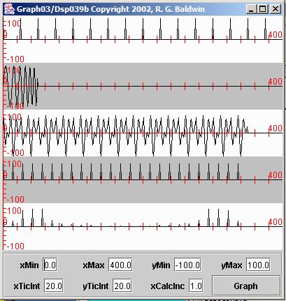 Figure 2 Output from the program named Dsp039b.
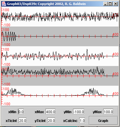 Figure 3 Output from the program named Dsp039c